Expressions
To compute on the language, we first need to understand its structure.
Learning objectives:
- Capture code expressions
- Inspect expressions
- Define expressions
- Modify expressions
- Generate/Automate expressions
expr captures code without executing
- Distinguishes the operation from the result
eval evaluates the code expression
Note
This chapter focuses on capturing and inspecting the operation. eval will be discussed more in chapters 19 and 20.
ast parses and identifies the parts of an expression
- Expressions are also called abstract syntax trees (ASTs) because of the hierarchical structure and natural tree representation.
The leaves, branches, and colors from ast identify expression data structures
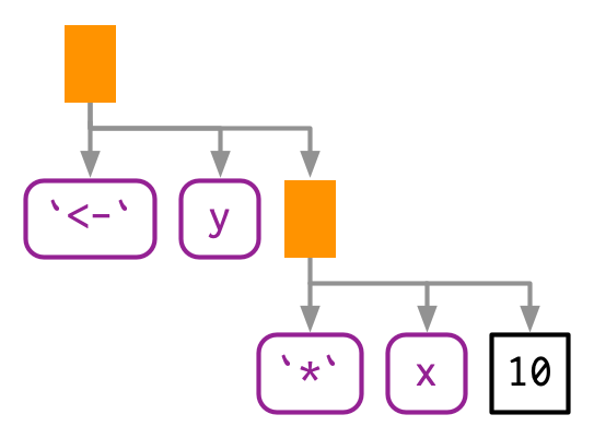
- Also called scalars
- Found in
astleaves - Leaves have black borders and sharp corners
- Identify with
rlang::is_syntactic_literal
- Found in
astleaves - Leaves have purple borders and rounded corners
- Identify with
is.nameoris.symbol - Convert strings to symbols with
rlang::symorrlang::syms - Convert a symbol to a string with
rlang::as_stringoras.character
- Found in
astbranches. - Branches are orange rectangles
- First child is the function call name
- Subsequent children are arguments to the function call
- Calls behave as lists
typeofandstrreturn “language” for call objects
Expressions and lists have similar memory mapping
#> [1] 3#> [1] FALSE#> [1] "0x1d950654c40"#> [1] "0x1d94815bff0"#> [1] "0x1d948b7b9e0"#> [1] "0x1d950654ce8"#> [1] "0x1d94815bff0" "0x1d948b7b9e0" "0x1d950654ce8"Expressions can be modified using list subsetting
#> [1] "<000001D95238AD28>"#> 10 * 2#> tracemem[0x000001d95238ad28 -> 0x000001d9545baf90]: eval eval withVisible withCallingHandlers eval eval with_handlers doWithOneRestart withOneRestart withRestartList doWithOneRestart withOneRestart withRestartList withRestarts <Anonymous> evaluate in_dir in_input_dir eng_r block_exec call_block process_group withCallingHandlers with_options <Anonymous> process_file <Anonymous> <Anonymous> execute .main#> 4 * 2Simple expressions can be generated using call2, parse_expr, or expr_text
- Clunky when creating more complex expressions, see chapter 19 for more details
- parsing: String to expression
- More details and safer usage in chapter 19
base::parse(text argument) is equivalent torlang::parse_expr
- deparsing: Expression to string
base::deparseoutputs a vector when spanning lines- The ‘questioning’ lifecycle in the Help page is telling…
Complex expressions can be automated using expr and purrr::reduce
#> # A tibble: 5 × 1
#>   x
#>   <chr>
#> 1 a
#> 2 b
#> 3 c
#> 4 d
#> 5 e#> # A tibble: 7 × 1
#> x
#> <chr>
#> 1 a
#> 2 b
#> 3 c
#> 4 d
#> 5 e
#> 6 f
#> 7 gThere are specialised data structures to be aware of but have been mostly replaced
- Only seen when working with calls to the function
- But can treat it as a regular list
- You only need to care about the missing symbol if you’re programmatically creating functions with missing arguments
- Use
rlang::missing_arg() - The
...argument is associated with an empty symbol
- Only generated by
base::expressionandbase::parse - Their “advantage” is
base::evalworks across te elements, but this is confusing compared to evaluating across a list of expressions