Intro to OOP and base types

Learning objectives:

• Understand what OOP means–at the very least for R
• Know how to discern an object’s nature–base or OO–and type

John Chambers, creator of S programming language

Session Info

library("DiagrammeR")

utils::sessionInfo()

#> R version 4.5.1 (2025-06-13)
#> Platform: aarch64-apple-darwin20
#> Running under: macOS Sequoia 15.7.1
#> 
#> Matrix products: default
#> BLAS:   /Library/Frameworks/R.framework/Versions/4.5-arm64/Resources/lib/libRblas.0.dylib 
#> LAPACK: /Library/Frameworks/R.framework/Versions/4.5-arm64/Resources/lib/libRlapack.dylib;  LAPACK version 3.12.1
#> 
#> locale:
#> [1] en_US.UTF-8/en_US.UTF-8/en_US.UTF-8/C/en_US.UTF-8/en_US.UTF-8
#> 
#> time zone: Europe/London
#> tzcode source: internal
#> 
#> attached base packages:
#> [1] stats     graphics  grDevices utils     datasets  methods   base     
#> 
#> other attached packages:
#> [1] DiagrammeR_1.0.11
#> 
#> loaded via a namespace (and not attached):
#>  [1] digest_0.6.37      RColorBrewer_1.1-3 fastmap_1.2.0      xfun_0.53         
#>  [5] magrittr_2.0.4     glue_1.8.0         knitr_1.50         htmltools_0.5.8.1 
#>  [9] rmarkdown_2.30     cli_3.6.5          visNetwork_2.1.4   compiler_4.5.1    
#> [13] tools_4.5.1        evaluate_1.0.5     yaml_2.3.10        rlang_1.1.6       
#> [17] jsonlite_2.0.0     htmlwidgets_1.6.4

Why OOP is hard in R

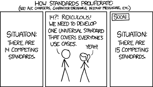
• Multiple OOP systems exist: S3, R6, S4, and (now/soon) S7.
• Multiple preferences: some users prefer one system; others, another.
• R’s OOP systems are different enough that prior OOP experience may not transfer well.

XKCD 927

Object Oriented Programming (OOP)

OOP: Big Idea - Polymorphism

Function has a single interface (outside), but contains (inside) several class-specific implementations.

# imagine a function with object x as an argument
# from the outside, users interact with the same function
# but inside the function, there are provisions to deal with objects of different classes
some_function <- function(x) {
  if is.numeric(x) {
    # implementation for numeric x
  } else if is.character(x) {
    # implementation for character x
  } ...
}

OOP: Big Idea - Polymorphism example

# data frame, with columns of different types
summary(palmerpenguins::penguins[, 1:4])

#>       species          island    bill_length_mm  bill_depth_mm  
#>  Adelie   :152   Biscoe   :168   Min.   :32.10   Min.   :13.10  
#>  Chinstrap: 68   Dream    :124   1st Qu.:39.23   1st Qu.:15.60  
#>  Gentoo   :124   Torgersen: 52   Median :44.45   Median :17.30  
#>                                  Mean   :43.92   Mean   :17.15  
#>                                  3rd Qu.:48.50   3rd Qu.:18.70  
#>                                  Max.   :59.60   Max.   :21.50  
#>                                  NA's   :2       NA's   :2

Improving summary for character vectors

summary on character vectors is current pretty useless.

summary(c("Adelie", "Adelie", "Chinstrap"))

#>    Length     Class      Mode 
#>         3 character character

Improvements are in the works (GitHub, bugzilla).

OOP: Big Idea - Polymorphism example

# statistical model
lin_fit <- lm(mpg ~ hp, data = mtcars)
summary(lin_fit)

#> 
#> Call:
#> lm(formula = mpg ~ hp, data = mtcars)
#> 
#> Residuals:
#>     Min      1Q  Median      3Q     Max 
#> -5.7121 -2.1122 -0.8854  1.5819  8.2360 
#> 
#> Coefficients:
#>             Estimate Std. Error t value Pr(>|t|)    
#> (Intercept) 30.09886    1.63392  18.421  < 2e-16 ***
#> hp          -0.06823    0.01012  -6.742 1.79e-07 ***
#> ---
#> Signif. codes:  0 '***' 0.001 '**' 0.01 '*' 0.05 '.' 0.1 ' ' 1
#> 
#> Residual standard error: 3.863 on 30 degrees of freedom
#> Multiple R-squared:  0.6024, Adjusted R-squared:  0.5892 
#> F-statistic: 45.46 on 1 and 30 DF,  p-value: 1.788e-07

OOP: Big Idea - Encapsulation

2. Encapsulation. Function “encapsulates”–that is, encloses in an inviolate capsule–both data and how it acts on data. The user doesn’t need to worry about details of an object because they are encapsulated behind a standard interface.

REST API comparison

Think of a REST API: a client interacts with with an API only through a set of discrete endpoints (i.e., things to get or set), but the server does not otherwise give access to its internal workings or state. Like with an API, this creates a separation of concerns: OOP functions take inputs and yield results; users only consume those results.

Objects have class

• Class defines:
  • Method (i.e., what can be done with object)
  • Fields (i.e., data that defines an instance of the class)
• Objects are an instance of a class

A class defines what an object is and methods describe what that object can do.

Class is inherited

• Class is defined:
  • By an object’s class (e.g., ordered factor)
  • By the parent of the object’s class (e.g., factor)
• Inheritance matters for method dispatch
  • If a method is defined for an object’s class, use that method
  • If an object doesn’t have a method, use the method of the parent class
  • The process of finding a method, is called dispatch

OOP in R

OOP in R: Two Paradigms

1. Encapsulated OOP

• Methods belong to objects or classes
• Method calls typically look like object.method(arg1, arg2)

• Calls communicate encapsulation, since form follows function
  • Form: object.method(arg1, arg2)
  • Function: for object, apply method for object’s class with arguments arg1 and arg2

OOP in R: Two Paradigms

2. Functional OOP

• Methods belong to “generic” functions
• From the outside, look like regular functions: generic(object, arg2, arg3)
• From the inside, components are also functions

Concept Map

Mermaid code

DiagrammeR::mermaid("
graph TB

OOP --> encapsulated_OOP
OOP --> functional_OOP

functional_OOP --> S3
functional_OOP --> S4

encapsulated_OOP --> R6
encapsulated_OOP --> RC
")

Functional OOP in base R

• S3
• S4

• Paradigm: functional OOP
• Noteworthy: R’s first OOP system
• Use case: low-cost solution for common problems
• Downsides: no guarantees

• Paradigm: functional OOP
• Noteworthy: rewrite of S3, used by Bioconductor
• Use case: “more guarantees and greater encapsulation” than S3
• Downsides: higher setup cost than S3

Encapsulated OOP in base R

• RC
  • Paradigm: encapsulated OOP
  • Noteworthy: special type of S4 object is mutable–in other words, that can be modified in place (instead of R’s usual copy-on-modify behavior)
  • Use cases: problems that are hard to tackle with functional OOP (in S3 and S4)
  • Downsides: harder to reason about (because of modify-in-place logic)

OOP in packages (various paradigms)

• R6
• S7
• proto
• R.oo

• Paradigm: encapsulated OOP
• Noteworthy: resolves issues with RC

• Paradigm: functional OOP
• Noteworthy:
  • best parts of S3 and S4 - ease of S3 with power of S4
  • Recently adopted in ggplot2 >= v4.0.0
  • See more in rstudio::conf(2022) talk and the S7 website
• Longer-term plan to incorporate into base R

• Paradigm: prototype OOP
• Noteworthy: OOP style used in ggplot2 < v4.0.0.

• Paradigm: hybrid functional and encapsulated (?)

sloop R package

“Sail the seas of OOP”

• S Language Object-Oriented Programming

Sloop John B ship (left) and Beach Boys album cover (right)

Use sloop::otype to determine OOP system

library(sloop)
otype(1:10)

#> [1] "base"

otype(mtcars)

#> [1] "S3"

mle_obj <- stats4::mle(function(x = 1) (x - 2) ^ 2)
otype(mle_obj)

#> [1] "S4"

Base types

Everything is an object, but not everything is object oriented

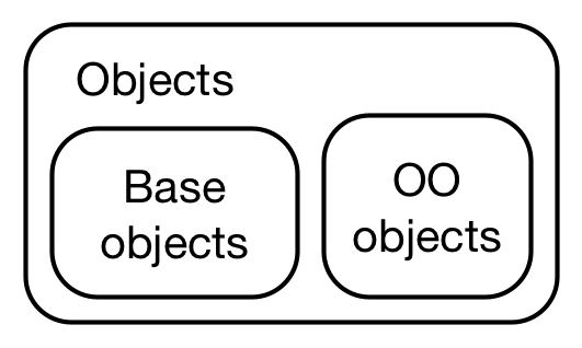
base objects and OO objects are different subsets of objects

You can use functions to determine if object is base or OOP

• base::is.object(): TRUE/FALSE for OOP
• sloop::otype(): gives object type: "base", "S3", etc.

# Example 1: a base object
is.object(1:10)

#> [1] FALSE

sloop::otype(1:10)

#> [1] "base"

# Example 2: an OO object
is.object(mtcars)

#> [1] TRUE

sloop::otype(mtcars)

#> [1] "S3"

OO objects have a “class” attribute, base objects do not

# base object has no class attribute
M <- matrix(1:4, 2)
attr(M, "class")

#> NULL

# OO object has one or more classes
attr(mtcars, "class")

#> [1] "data.frame"

attr(palmerpenguins::penguins, "class")

#> [1] "tbl_df"     "tbl"        "data.frame"

Be careful with class()

class() gives misleading results for base objects.

It is not enough to call class() on an object to determine if it is base or OO, as this will return the implicit class (rather than NULL) when there is no class attribute (i.e. "matrix", "array", "function", "numeric" or result of typeof()):

class(1:10)

#> [1] "integer"

class(M)

#> [1] "matrix" "array"

sloop::s3_class() is safer, as it returns the implicit class that the S3 and S4 systems will use to pick methods

s3_class(M)

#> [1] "matrix"  "integer" "numeric"

What about types?

Only OO objects have a “class” attribute, but every object–whether base or OO–has a base type

There are 25 types.

They are most important in C code, so often see them called by their C type names, e.g. NILSXP for NULL.

Type examples

• Vectors
• Functions
• Environments
• S4
• Language components

typeof(NULL) # NILSXP

#> [1] "NULL"

typeof(c("a", "b", "c")) # STRSXP

#> [1] "character"

typeof(mtcars) # VECSXP

#> [1] "list"

typeof(1) # REALSXP

#> [1] "double"

typeof(1L) # INTSXP

#> [1] "integer"

typeof(1i) # CPLXSXP

#> [1] "complex"

# "normal" function
my_fun <- function(x) { x + 1 }
typeof(my_fun) # CLOSXP

#> [1] "closure"

# internal function
typeof(`[`) # SPECIALSXP

#> [1] "special"

# primitive function
typeof(sum) # BUILTINSXP

#> [1] "builtin"

typeof(globalenv()) # ENVSXP

#> [1] "environment"

mle_obj <- stats4::mle(function(x = 1) (x - 2) ^ 2)
typeof(mle_obj) # S4SXP

#> [1] "S4"

typeof(quote(a)) # SYMSXP

#> [1] "symbol"

typeof(quote(a + 1)) # LANGSXP

#> [1] "language"

typeof(formals(my_fun)) # LISTSXP

#> [1] "pairlist"

Concept Map

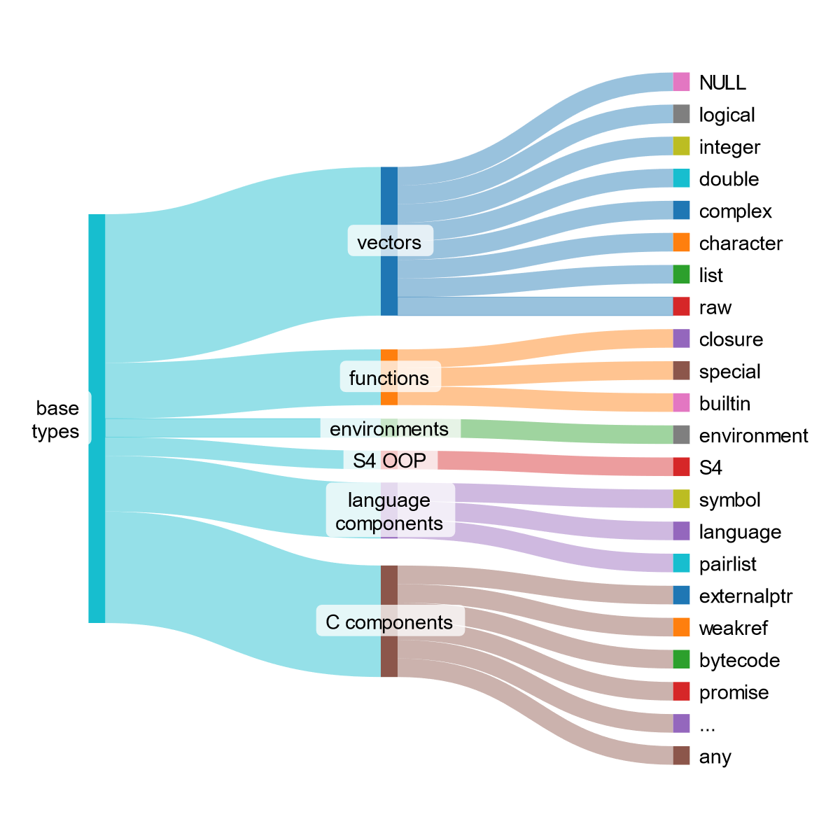
Base types in R

Sankey graph code

The graph above was made with SankeyMATIC

// toggle "Show Values"
// set Default Flow Colors from "each flow's Source"

base\ntypes [8] vectors
base\ntypes [3] functions
base\ntypes [1] environments
base\ntypes [1] S4 OOP
base\ntypes [3] language\ncomponents
base\ntypes [6] C components

vectors [1] NULL
vectors [1] logical
vectors [1] integer
vectors [1] double
vectors [1] complex
vectors [1] character
vectors [1] list
vectors [1] raw

functions [1] closure
functions [1] special
functions [1] builtin

environments [1] environment

S4 OOP [1] S4

language\ncomponents [1] symbol
language\ncomponents [1] language
language\ncomponents [1] pairlist

C components [1] externalptr
C components [1] weakref
C components [1] bytecode
C components [1] promise
C components [1] ...
C components [1] any

Be careful about the numeric type

R uses “numeric” to mean three slightly different things:

1. Alias for double

2. In S3 and S4, as shorthand for integer or double

3. is.numeric() tests for objects that behave like numbers

Advanced R consistently uses numeric to mean an object of type integer or double.

1: “numeric” is treated as synonymous for double

# create a double and integeger objects
one <- 1
oneL <- 1L
typeof(one)

#> [1] "double"

typeof(oneL)

#> [1] "integer"

# check their type after as.numeric()
one |> as.numeric() |> typeof()

#> [1] "double"

oneL |> as.numeric() |> typeof()

#> [1] "double"

2: in S3 and S4

“numeric” is taken as either integer or double, and used when choosing methods:

sloop::s3_class(1)

#> [1] "double"  "numeric"

sloop::s3_class(1L)

#> [1] "integer" "numeric"

3: testing behaviour

typeof(factor("x"))

#> [1] "integer"

is.numeric(factor("x"))

#> [1] FALSE