Function factories

Learning objectives:

By the end of today’s session, you will be able to:

• Identify function factories
• Understand how function factories work
• Learn about non-obvious combination of function features
• Generate a family of functions from data

What is a function factory?

• A function factory is a function that makes (returns) functions

• Factory made function are manufactured functions

# create a function factory
power1 <- function(exp) {
  function(x) {
    x^exp
  }
}

# create manufactured functions
square <- power1(2)

cube <- power1(3)

# execute manufactured functions
square(2)
#> 4

cube(2)
#> 8

• A function that, in its body, returns a function is by definition a function factory

• Of the three main functional programming tools (functionals, function factories, and function operators), function factories are the least used

Why function factories work

Function factories are powered by three features of the R language:

1. R has first-class functions

2. R functions capture the environment in which they are created

3. R functions create a new execution environment

env_print(square)

#> <environment: 0x55855d84aa38>
#> Parent: <environment: global>
#> Bindings:
#> • exp: <dbl>

env_print(cube)

#> <environment: 0x55855d8a0c68>
#> Parent: <environment: global>
#> Bindings:
#> • exp: <dbl>

• A language with first-class functions means the functions are objects that can be copied, bound, etc.

• When they are created, manufactured functions capture the environment of the function factory

• Manufactured functions have separate environments

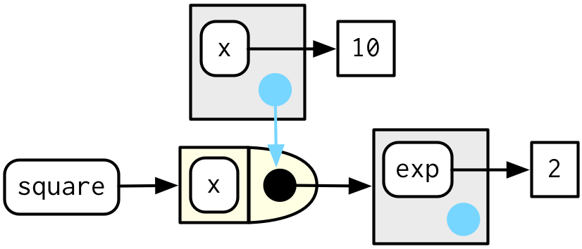
Diagramming function factories

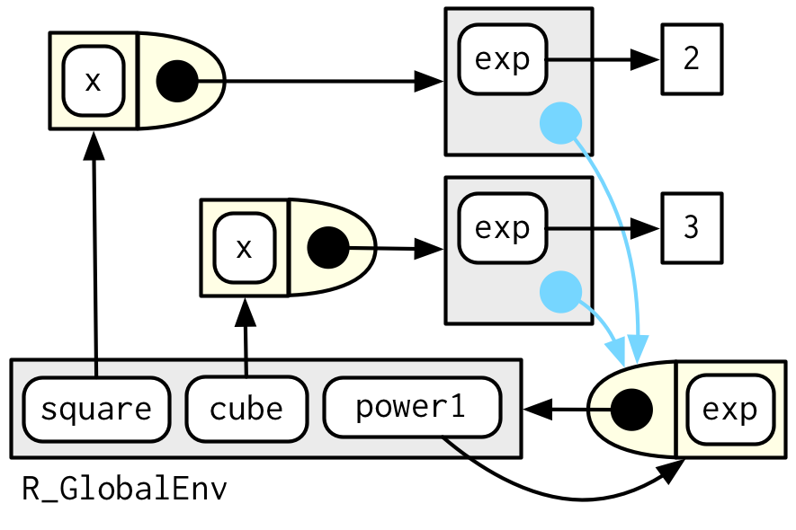
Diagramming function factories

Forcing evaluation

• Beware of changing bindings between creation and execution of manufactured functions

x <- 2
square <- power1(x)
x <- 3
square(2)
#> [1] 8

power2 <- function(exp) {
  force(exp)
  function(x) {
    x^exp
  }
}

x <- 2
square <- power2(x)
x <- 3
square(2)
#> [1] 4

• As per lazy evaluation, x is evaluated for the first time when square(2) is called and at the time of evaluation, x, the exponent, is equal to 3

• Use force() to force eager evaluation and avoid this type of bug introduced by lazy evaluation

• Alternatively, use any other function to force the evaluation of the variable x during the creation of the manufactured function

• This issue of lazy evaluation only applies for variables (e.g. running power2(2) is eagerly evaluated)

Stateful functions

new_counter <- function() {
  i <- 0
  function() {
    i <<- i + 1
    i
  }
}

counter_one <- new_counter()
counter_two <- new_counter()

counter_one()
#> [1] 1
counter_one()
#> [1] 2
counter_two()
#> [1] 1

• The manufactured functions create distinct enclosures of the function factory environment

• As soon as your function starts managing the state of multiple variables, it’s better to switch to an object-oriented system like R6

Garbage collection

• Manufactured functions hold on to variables in the enclosed function factory’s environment

f1 <- function(n) {
  x <- runif(n)
  m <- mean(x)
  function() m
}

g1 <- f1(1e6)
lobstr::obj_size(g1)
#> 8.00 MB

f2 <- function(n) {
  x <- runif(n)
  m <- mean(x)
  rm(x)
  function() m
}

g2 <- f2(1e6)
lobstr::obj_size(g2)
#> 504 B

Function factories + functionals

• Combine functionals and function factories to turn data into many functions.

names <- list(
  square = 2,
  cube = 3,
  root = 1 / 2,
  cuberoot = 1 / 3,
  reciprocal = -1
)
funs <- purrr::map(names, power1)

funs$root(64)
#> [1] 8
funs$root
#> function (x)
#> {
#>     x^exp
#> }
#> <bytecode: 0x55ce583c7828>
#> <environment: 0x55ce5a61cd60>

Avoid the funs$ prefix with

with(funs, root(100))
#> [1] 10

attach(funs)
#> The following objects are
#> masked _by_ .GlobalEnv:
#>
#>     cube, square
root(100)
#> [1] 10

rlang::env_bind(
  globalenv(),
  !!!funs
)

root(100)
#> [1] 10