Functions
Learning objectives
- How to make functions in R
- What are the parts of a function
- Nested functions
How to make a simple function in R
Function components
Functions have three parts, formals(), body(), and environment().
Example: coffee rations
#> {
#> avg <- summarise(filter(coffee_ratings, species == species),
#> mean = mean(total_cup_points))
#> return(avg)
#> }Functions uses attributes, one attribute used by base R is srcref, short for source reference. It points to the source code used to create the function. It contains code comments and other formatting.
Primitive functions
Are the core function in base R, such as sum()
Type of primitives:
- builtin
- special
These core functions have components to NULL.
Anonymous functions
If you don’t provide a name to a function
#> $mpg
#> [1] 25
#>
#> $cyl
#> [1] 3Invoking a function
#> # A tibble: 1 × 1
#>    mean
#>   <dbl>
#> 1 82.1do.call is used a lot with apply’s family
Function composition
#> [1] 0.2905932#> [1] 0.2905932More about functions insights
Lexical scoping
Rules
- Name masking
- Functions versus variables
- A fresh start
- Dynamic lookup
Name masking
Save us from our polluted global environment!
#> [1] "test" "bacon"#> [1] "test" "2"Note: also applied for functions names
Functions versus variables
Caution
Do not be too smart!
Fresh start:
Dynamic scoping:
“When”: R looks for the value when the function is run
This function
Debugging
You can change the function’s environment to an environment which contains nothing:
Lazy Evaluation:
Important
function arguments are only evaluated when accessed
Promises
See you at chapter 20!
Promises: multiple definitions?
Promises in Shiny
Default arguments
Arguments defined by other arguments or variables in Functions
Caution
Not recommended by Hadley!
Missing arguments
missing() checks if an argument is missing (TRUE/FALSE) then you can “branch” according to it
Caution
Do not be like sample() !
… (dot-dot-dot)
Example
#> List of 2
#>  $ y: num 2
#>  $ z: num 3
Used a lot with higher ordered functions!
Exiting a function
Implicit or explicit returns
Invisibility (
<-most famous function that returns an invisible value)stop()to stop a function with an error.Exit handlers (
on.exit())
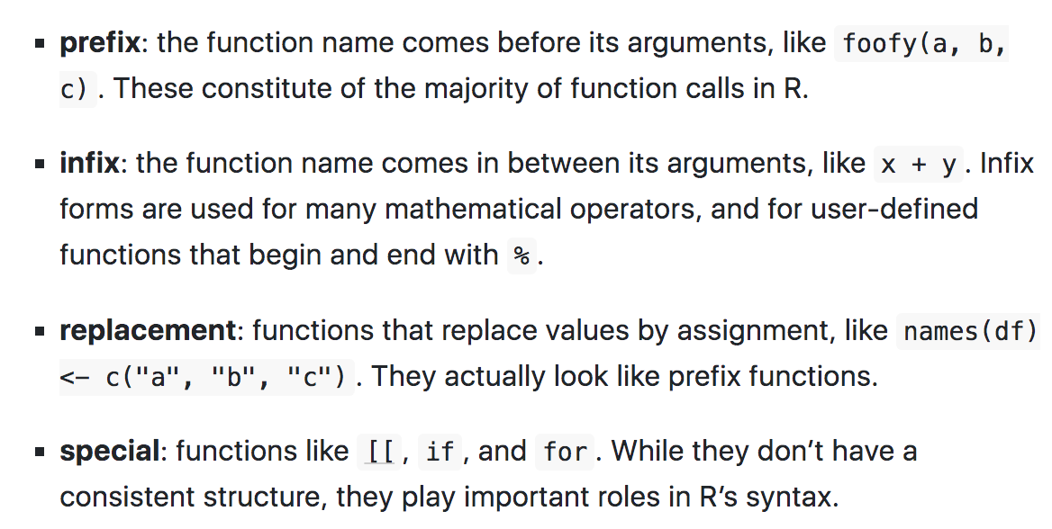
Function forms
Everything that exists is an object. Everything that happens is a function call. — John Chambers
Case Study: SIR model function
This is an interesting example taken from a course on Coursera: Infectious disease modelling-ICL
The purpose of this example is to show how to make a model passing through making a function.
First we need to load some useful libraries:
Then set the model inputs:
- population size (N)
- number of susceptable (S)
- infected (I)
- recovered (R)
And add the model parameters:
- infection rate (\(\beta\))
- recovery rate (\(\gamma\))
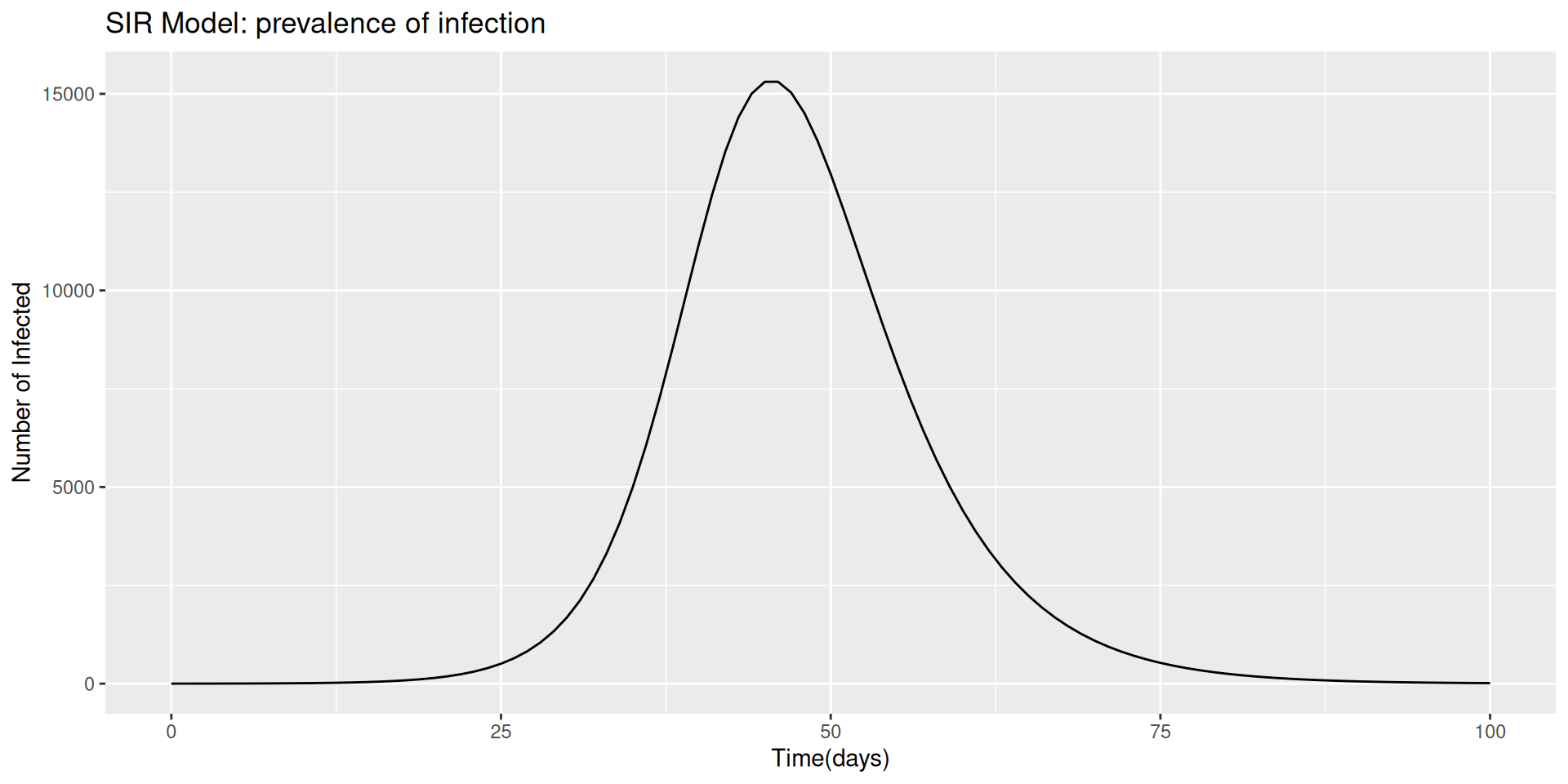
Then we set the time as an important factor, which defines the length of time we are looking at this model run. It is intended as the time range in which the infections spread out, let’s say that we are aiming to investigate an infection period of 100 days.
Finally, we set up the SIR model, the susceptable, infected and recovered model. How do we do that is passing the paramenters through a function of the time, and state.
Within the model function we calculate one more paramenter, the force of infection: \(\lambda\)
Once we have our SIR model function ready, we can calculate the output of the model, with the help of the function ode() from {deSolve} package.
#>   time        S        I         R
#> 1    0 99999.00 1.000000 0.0000000
#> 2    1 99998.43 1.284018 0.2840252
#> 3    2 99997.70 1.648696 0.6487171
#> 4    3 99996.77 2.116939 1.1169863
#> 5    4 99995.56 2.718152 1.7182450
#> 6    5 99994.02 3.490086 2.4902600
In addition to our builtin SIR model function we can have a look at:
It solves Ordinary Differential Equations.
#> function (y, times, func, parms, method = c("lsoda", "lsode",
#>     "lsodes", "lsodar", "vode", "daspk", "euler", "rk4", "ode23",
#>     "ode45", "radau", "bdf", "bdf_d", "adams", "impAdams", "impAdams_d",
#>     "iteration"), ...)
#> {
#>     if (is.null(method))
#>         method <- "lsoda"
#>     if (is.list(method)) {
#>         if (!inherits(method, "rkMethod"))
#>             stop("'method' should be given as string or as a list of class 'rkMethod'")
#>         out <- rk(y, times, func, parms, method = method, ...)
#>     }
#>     else if (is.function(method))
#>         out <- method(y, times, func, parms, ...)
#>     else if (is.complex(y))
#>         out <- switch(match.arg(method), vode = zvode(y, times,
#>             func, parms, ...), bdf = zvode(y, times, func, parms,
#>             mf = 22, ...), bdf_d = zvode(y, times, func, parms,
#>             mf = 23, ...), adams = zvode(y, times, func, parms,
#>             mf = 10, ...), impAdams = zvode(y, times, func, parms,
#>             mf = 12, ...), impAdams_d = zvode(y, times, func,
#>             parms, mf = 13, ...))
#>     else out <- switch(match.arg(method), lsoda = lsoda(y, times,
#>         func, parms, ...), vode = vode(y, times, func, parms,
#>         ...), lsode = lsode(y, times, func, parms, ...), lsodes = lsodes(y,
#>         times, func, parms, ...), lsodar = lsodar(y, times, func,
#>         parms, ...), daspk = daspk(y, times, func, parms, ...),
#>         euler = rk(y, times, func, parms, method = "euler", ...),
#>         rk4 = rk(y, times, func, parms, method = "rk4", ...),
#>         ode23 = rk(y, times, func, parms, method = "ode23", ...),
#>         ode45 = rk(y, times, func, parms, method = "ode45", ...),
#>         radau = radau(y, times, func, parms, ...), bdf = lsode(y,
#>             times, func, parms, mf = 22, ...), bdf_d = lsode(y,
#>             times, func, parms, mf = 23, ...), adams = lsode(y,
#>             times, func, parms, mf = 10, ...), impAdams = lsode(y,
#>             times, func, parms, mf = 12, ...), impAdams_d = lsode(y,
#>             times, func, parms, mf = 13, ...), iteration = iteration(y,
#>             times, func, parms, ...))
#>     return(out)
#> }
#> <bytecode: 0x0000021ebc6bc708>
#> <environment: namespace:deSolve>With the help of the {reshape2} package we use the function melt() to reshape the output:
#>   time variable    value
#> 1    0        S 99999.00
#> 2    1        S 99998.43
#> 3    2        S 99997.70
#> 4    3        S 99996.77
#> 5    4        S 99995.56
#> 6    5        S 99994.02
The same as usign pivot_longer() function.
Before to proceed with the visualization of the SIR model output we do a bit of investigations.
What if we want to see how melt() function works?
What instruments we can use to see inside the function and understand how it works?
Using just the function name melt or structure() function with melt as an argument, we obtain the same output. To select just the argument of the function we can do args(melt)
#> function (data, ..., na.rm = FALSE, value.name = "value")
#> {
#>     UseMethod("melt", data)
#> }
#> <bytecode: 0x0000021ebb4c0c10>
#> <environment: namespace:reshape2>“R functions simulate a closure by keeping an explicit reference to the environment that was active when the function was defined.”
ref: closures
Try with methods(), or print(methods(melt)): Non-visible functions are asterisked!
The S3 method name is followed by an asterisk * if the method definition is not exported from the package namespace in which the method is defined.
#> [1] melt.array*      melt.data.frame* melt.default*    melt.list*
#> [5] melt.matrix*     melt.table*
#> see '?methods' for accessing help and source code#> [1] [ aperm as.data.frame as_tibble Axis
#> [6] coerce initialize lines melt plot
#> [11] points print show slotsFromS3 summary
#> [16] tail
#> see '?methods' for accessing help and source codeWe can access to some of the above calls with getAnywhere(), for example here is done for “melt.data.frame”:
#> A single object matching 'melt.data.frame' was found
#> It was found in the following places
#>   registered S3 method for melt from namespace reshape2
#>   namespace:reshape2
#> with value
#>
#> function (data, id.vars, measure.vars, variable.name = "variable",
#>     ..., na.rm = FALSE, value.name = "value", factorsAsStrings = TRUE)
#> {
#>     vars <- melt_check(data, id.vars, measure.vars, variable.name,
#>         value.name)
#>     id.ind <- match(vars$id, names(data))
#>     measure.ind <- match(vars$measure, names(data))
#>     if (!length(measure.ind)) {
#>         return(data[id.vars])
#>     }
#>     args <- normalize_melt_arguments(data, measure.ind, factorsAsStrings)
#>     measure.attributes <- args$measure.attributes
#>     factorsAsStrings <- args$factorsAsStrings
#>     valueAsFactor <- "factor" %in% measure.attributes$class
#>     df <- melt_dataframe(data, as.integer(id.ind - 1), as.integer(measure.ind -
#>         1), as.character(variable.name), as.character(value.name),
#>         as.pairlist(measure.attributes), as.logical(factorsAsStrings),
#>         as.logical(valueAsFactor))
#>     if (na.rm) {
#>         return(df[!is.na(df[[value.name]]), ])
#>     }
#>     else {
#>         return(df)
#>     }
#> }
#> <bytecode: 0x0000021eb6346070>
#> <environment: namespace:reshape2>
References:
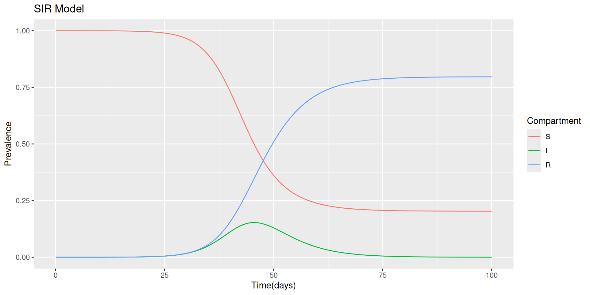
Going back to our model output visualization.