Vectors

Learning objectives:

Learn about different types of vectors and their attributes
Navigate through vector types and their value types
Venture into factors and date-time objects
Discuss the differences between data frames and tibbles
Do not get absorbed by the NA and NULL black hole

Session Info

library("dplyr")
library("gt")
library("palmerpenguins")

Session Info

utils::sessionInfo()

#> R version 4.5.1 (2025-06-13 ucrt)
#> Platform: x86_64-w64-mingw32/x64
#> Running under: Windows 11 x64 (build 26100)
#> 
#> Matrix products: default
#>   LAPACK version 3.12.1
#> 
#> locale:
#> [1] LC_COLLATE=English_United States.utf8 
#> [2] LC_CTYPE=English_United States.utf8   
#> [3] LC_MONETARY=English_United States.utf8
#> [4] LC_NUMERIC=C                          
#> [5] LC_TIME=English_United States.utf8    
#> 
#> time zone: America/Chicago
#> tzcode source: internal
#> 
#> attached base packages:
#> [1] stats     graphics  grDevices utils     datasets  methods   base     
#> 
#> other attached packages:
#> [1] palmerpenguins_0.1.1 gt_1.0.0             dplyr_1.1.4         
#> 
#> loaded via a namespace (and not attached):
#>  [1] digest_0.6.37     R6_2.6.1          fastmap_1.2.0     tidyselect_1.2.1 
#>  [5] xfun_0.53         magrittr_2.0.3    glue_1.8.0        tibble_3.3.0     
#>  [9] knitr_1.50        pkgconfig_2.0.3   htmltools_0.5.8.1 rmarkdown_2.29   
#> [13] generics_0.1.4    lifecycle_1.0.4   xml2_1.3.8        cli_3.6.5        
#> [17] vctrs_0.6.5       compiler_4.5.1    tools_4.5.1       pillar_1.11.0    
#> [21] evaluate_1.0.4    yaml_2.3.10       rlang_1.1.6       jsonlite_2.0.0   
#> [25] keyring_1.4.1

Aperitif

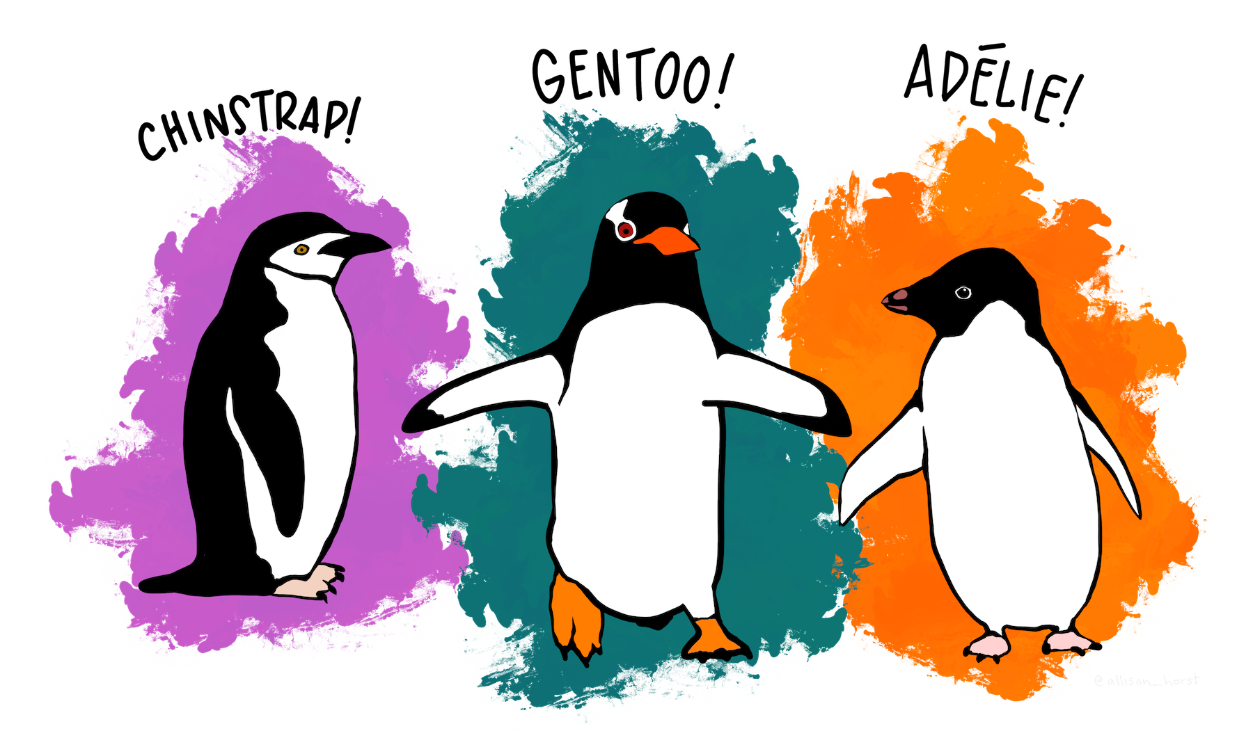
Palmer Penguins

Counting Penguins

Consider this code to count the number of Gentoo penguins in the penguins data set. We see that there are 124 Gentoo penguins.

sum("Gentoo" == penguins$species)
# output: 124

In

One subtle error can arise in trying out %in% here instead.

species_vector <- penguins |> select(species)
print("Gentoo" %in% species_vector)
# output: FALSE

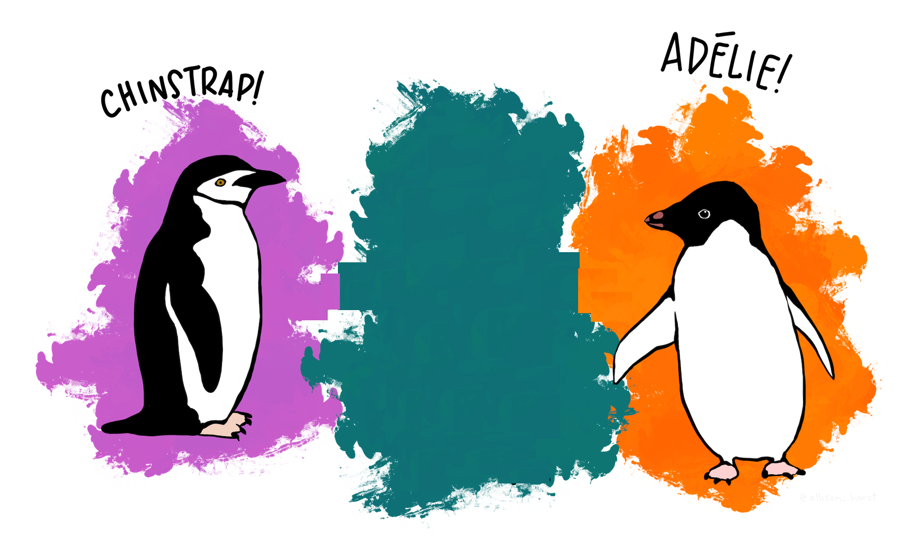
Where did the penguins go?

Fix: base R

species_unlist <- penguins |> select(species) |> unlist()
print("Gentoo" %in% species_unlist)
# output: TRUE

Fix: dplyr

species_pull <- penguins |> select(species) |> pull()
print("Gentoo" %in% species_pull)
# output: TRUE

Motivation

What are the different types of vectors?
How does this affect accessing vectors?

Side Quest: Looking up the %in% operator

If you want to look up the manual pages for the %in% operator with the ?, use backticks:

?`%in%`

and we find that %in% is a wrapper for the match() function.

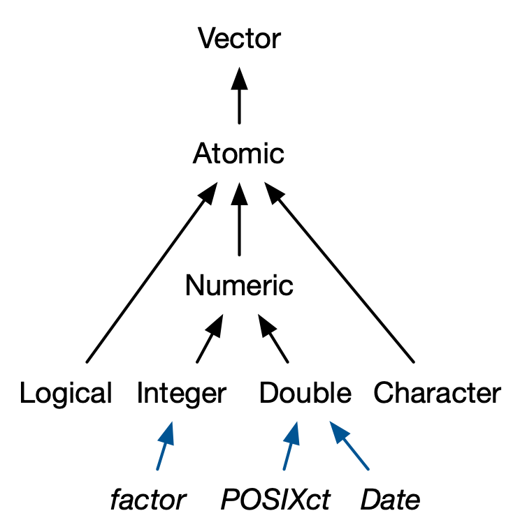
Types of Vectors

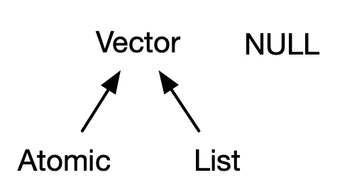
Image Credit: Advanced R

Two main types:

Atomic: Elements all the same type.
List: Elements are different Types.

Closely related but not technically a vector:

NULL: Null elements. Often length zero.

Types of Atomic Vectors (1/2)

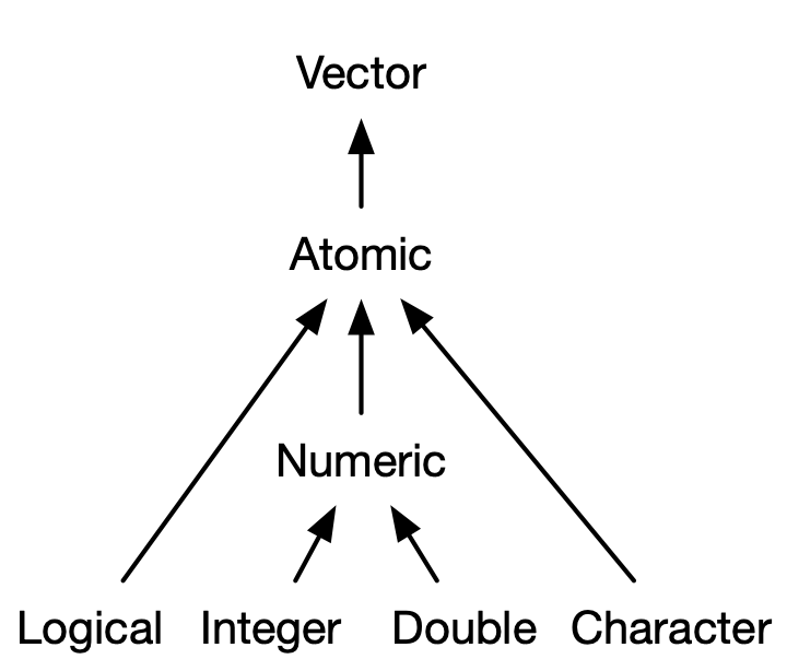
Image Credit: Advanced R

Types of Atomic Vectors (2/2)

Logical: True/False
Integer: Numeric (discrete, no decimals)
Double: Numeric (continuous, decimals)
Character: String

Vectors of Length One

Scalars are vectors that consist of a single value.

Logicals

lgl1 <- TRUE
lgl2 <- T #abbreviation for TRUE
lgl3 <- FALSE
lgl4 <- F #abbreviation for FALSE

Doubles

# integer, decimal, scientific, or hexidecimal format
dbl1 <- 1
dbl2 <- 1.234 # decimal
dbl3 <- 1.234e0 # scientific format
dbl4 <- 0xcafe # hexidecimal format

Integers

Integers must be followed by L and cannot have fractional values

int1 <- 1L
int2 <- 1234L
int3 <- 1234e0L
int4 <- 0xcafeL

Pop Quiz: Why “L” for integers?

Wickham notes that the use of L dates back to the C programming language and its “long int” type for memory allocation.

Strings

Strings can use single or double quotes and special characters are escaped with

str1 <- "hello" # double quotes
str2 <- 'hello' # single quotes
str3 <- "مرحبًا" # Unicode
str4 <- "\U0001f605" # sweaty_smile 😅

Longer 1/2

There are several ways to make longer vectors:

1. With single values inside c() for combine.

lgl_var <- c(TRUE, FALSE)
int_var <- c(1L, 6L, 10L)
dbl_var <- c(1, 2.5, 4.5)
chr_var <- c("these are", "some strings")

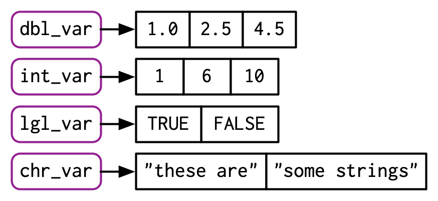
Image Credit: Advanced R

Longer 2/2

2. With other vectors

c(c(1, 2), c(3, 4)) # output is not nested

#> [1] 1 2 3 4

Type and Length

We can determine the type of a vector with typeof() and its length with length()

Types of Atomic Vectors¹
name	value	typeof()	length()
lgl_var	TRUE, FALSE	logical	2
int_var	1L, 6L, 10L	integer	3
dbl_var	1, 2.5, 4.5	double	3
chr_var	'these are', 'some strings'	character	2
¹ Source: https://adv-r.hadley.nz/index.html

Side Quest: Penguins

typeof(penguins$species)

#> [1] "integer"

class(penguins$species)

#> [1] "factor"

typeof(species_unlist)

#> [1] "integer"

class(species_unlist)

#> [1] "factor"

typeof(species_pull)

#> [1] "integer"

class(species_pull)

#> [1] "factor"

Missing values: Contagion

For most computations, an operation over values that includes a missing value yields a missing value (unless you’re careful)

# contagion
5*NA

#> [1] NA

sum(c(1, 2, NA, 3))

#> [1] NA

Missing values: Contagion Exceptions

NA ^ 0
#> [1] 1
NA | TRUE
#> [1] TRUE
NA & FALSE
#> [1] FALSE

Innoculation

sum(c(1, 2, NA, 3), na.rm = TRUE)
# output: 6

To search for missing values use is.na()

x <- c(NA, 5, NA, 10)
x == NA
# output: NA NA NA NA [BATMAN!]

is.na(x)
# output: TRUE FALSE TRUE FALSE

Missing Values: NA Types

Each type has its own NA type

Logical: NA
Integer: NA_integer
Double: NA_double
Character: NA_character

This may not matter in many contexts.

Can matter for operations where types matter like dplyr::if_else().

Testing (1/2)

What type of vector is.*() it?

Test data type:

Logical: is.logical()
Integer: is.integer()
Double: is.double()
Character: is.character()

Testing (2/2)

What type of object is it?

Don’t test objects with these tools:

is.vector()
is.atomic()
is.numeric()

They don’t test if you have a vector, atomic vector, or numeric vector; you’ll need to carefully read the documentation to figure out what they actually do (preview: attributes)

Side Quest: rlang `is_*()`

Maybe use {rlang}?

rlang::is_vector
rlang::is_atomic

# vector
rlang::is_vector(c(1, 2))

#> [1] TRUE

rlang::is_vector(list(1, 2))

#> [1] TRUE

# atomic
rlang::is_atomic(c(1, 2))

#> [1] TRUE

rlang::is_atomic(list(1, "a"))

#> [1] FALSE

See more here

Coercion

R follows rules for coercion: character → double → integer → logical
R can coerce either automatically or explicitly

Automatic

Two contexts for automatic coercion:

Combination
Mathematical

Coercion by Combination:

str(c(TRUE, "TRUE"))

#>  chr [1:2] "TRUE" "TRUE"

Coercion by Mathematical operations:

# imagine a logical vector about whether an attribute is present
has_attribute <- c(TRUE, FALSE, TRUE, TRUE)

# number with attribute
sum(has_attribute)

#> [1] 3

Explicit

Coercion of Atomic Vectors¹
name	value	as.logical()	as.integer()	as.double()	as.character()
lgl_var	TRUE, FALSE	TRUE FALSE	1 0	1 0	'TRUE' 'FALSE'
int_var	1L, 6L, 10L	TRUE TRUE TRUE	1 6 10	1 6 10	'1' '6' '10'
dbl_var	1, 2.5, 4.5	TRUE TRUE TRUE	1 2 4	1.0 2.5 4.5	'1' '2.5' '4.5'
chr_var	'these are', 'some strings'	NA NA	NA_integer	NA_double	'these are', 'some strings'
¹ Source: https://adv-r.hadley.nz/index.html

But note that coercion may fail in one of two ways, or both:

With warning/error
NAs

as.integer(c(1, 2, "three"))

#> [1]  1  2 NA

Exercises 1/5

How do you create raw and complex scalars?

Answer(s)

as.raw(42)
#> [1] 2a
charToRaw("A")
#> [1] 41
complex(length.out = 1, real = 1, imaginary = 1)
#> [1] 1+1i

Exercises 2/5

Test your knowledge of the vector coercion rules by predicting the output of the following uses of c():

c(1, FALSE)
c("a", 1)
c(TRUE, 1L)

Answer(s)

c(1, FALSE)      # will be coerced to double    -> 1 0
c("a", 1)        # will be coerced to character -> "a" "1"
c(TRUE, 1L)      # will be coerced to integer   -> 1 1

Exercises 3/5

Why is 1 == "1" true? Why is -1 < FALSE true? Why is "one" < 2 false?

Answer(s)

These comparisons are carried out by operator-functions (==, <), which coerce their arguments to a common type. In the examples above, these types will be character, double and character: 1 will be coerced to “1”, FALSE is represented as 0 and 2 turns into “2” (and numbers precede letters in lexicographic order (may depend on locale)).

Exercises 4/5

Why is the default missing value, NA, a logical vector? What’s special about logical vectors?

Answer(s)

The presence of missing values shouldn’t affect the type of an object. Recall that there is a type-hierarchy for coercion from character → double → integer → logical. When combining NAs with other atomic types, the NAs will be coerced to integer (NA_integer_), double (NA_real_) or character (NA_character_) and not the other way round. If NA were a character and added to a set of other values all of these would be coerced to character as well.

Exercises 5/5

Precisely what do is.atomic(), is.numeric(), and is.vector() test for?

Answer(s)

is.atomic() tests if an object is an atomic vector or is NULL (!). Atomic vectors are objects of type logical, integer, double, complex, character or raw.
is.numeric() tests if an object has type integer or double and is not of class factor, Date, POSIXt or difftime.
is.vector() tests if an object is a vector or an expression and has no attributes, apart from names. Vectors are atomic vectors or lists.

Attributes

Attributes are name-value pairs that attach metadata to an object (vector).

Name-value pairs: attributes have a name and a value
Metadata: not data itself, but data about the data

Getting and Setting

Three functions:

retrieve and modify single attributes with attr()
retrieve en masse with attributes()
set en masse with structure()

Single attribute

Use attr()

# some object
a <- c(1, 2, 3)

# set attribute
attr(x = a, which = "attribute_name") <- "some attribute"

# get attribute
attr(a, "attribute_name")

#> [1] "some attribute"

Multiple attributes

structure(): set multiple attributes, attributes(): get multiple attributes

a <- 1:3
attr(a, "x") <- "abcdef"
attr(a, "x")

#> [1] "abcdef"

attr(a, "y") <- 4:6
str(attributes(a))

#> List of 2
#>  $ x: chr "abcdef"
#>  $ y: int [1:3] 4 5 6

b <- structure(
  1:3, 
  x = "abcdef",
  y = 4:6
)
identical(a, b)

#> [1] TRUE

Why

Three particularly important attributes:

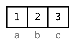
names - a character vector giving each element a name
dimension - (or dim) turns vectors into matrices and arrays
class - powers the S3 object system (we’ll learn more about this in chapter 13)

Most attributes are lost by most operations. Only two attributes are routinely preserved: names and dimension.

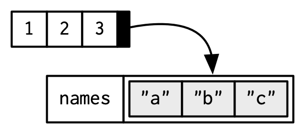
Names

~~Three~~ Four ways to name:

# (1) On creation: 
x <- c(A = 1, B = 2, C = 3)
x

#> A B C 
#> 1 2 3

# (2) Assign to names():
y <- 1:3
names(y) <- c("a", "b", "c")
y

#> a b c 
#> 1 2 3

# (3) Inline:
z <- setNames(1:3, c("a", "b", "c"))
z

#> a b c 
#> 1 2 3

rlang Names

# (4) Inline with {rlang}:
a <- 1:3
rlang::set_names(
  a,
  c("a", "b", "c")
)

#> a b c 
#> 1 2 3

Removing names

x <- unname(x) or names(x) <- NULL
Thematically but not directly related: labelled class vectors with haven::labelled()

Dimensions: `matrix()` and `array()`

# Two scalar arguments specify row and column sizes
x <- matrix(1:6, nrow = 2, ncol = 3)
x

#>      [,1] [,2] [,3]
#> [1,]    1    3    5
#> [2,]    2    4    6

# One vector argument to describe all dimensions
y <- array(1:12, c(2, 3, 2)) # rows, columns, no of arrays
y

#> , , 1
#> 
#>      [,1] [,2] [,3]
#> [1,]    1    3    5
#> [2,]    2    4    6
#> 
#> , , 2
#> 
#>      [,1] [,2] [,3]
#> [1,]    7    9   11
#> [2,]    8   10   12

Dimensions: assign to `dim()`

# You can also modify an object in place by setting dim()
z <- 1:6
dim(z) <- c(2, 3) # rows, columns
z

#>      [,1] [,2] [,3]
#> [1,]    1    3    5
#> [2,]    2    4    6

a <- 1:12
dim(a) <- c(2, 3, 2) # rows, columns, no of arrays
a

#> , , 1
#> 
#>      [,1] [,2] [,3]
#> [1,]    1    3    5
#> [2,]    2    4    6
#> 
#> , , 2
#> 
#>      [,1] [,2] [,3]
#> [1,]    7    9   11
#> [2,]    8   10   12

Functions for working with vectors, matrices and arrays (1/2):

Vector	Matrix	Array
`names()`	`rownames()`, `colnames()`	`dimnames()`
`length()`	`nrow()`, `ncol()`	`dim()`
`c()`	`rbind()`, `cbind()`	`abind::abind()`
—	`t()`	`aperm()`
`is.null(dim(x))`	`is.matrix()`	`is.array()`

Caution: Vector without dim set has NULL dimensions, not 1.
One dimension?

Functions for working with vectors, matrices and arrays (2/2):

str(1:3)                   # 1d vector
#>  int [1:3] 1 2 3
str(matrix(1:3, ncol = 1)) # column vector
#>  int [1:3, 1] 1 2 3
str(matrix(1:3, nrow = 1)) # row vector
#>  int [1, 1:3] 1 2 3
str(array(1:3, 3))         # "array" vector
#>  int [1:3(1d)] 1 2 3

Exercises 1/4

How is setNames() implemented? Read the source code.

Answer(s)

setNames <- function(object = nm, nm) {
  names(object) <- nm
  object
}

Data arg 1st = works well with pipe.
1st arg is optional

setNames( , c("a", "b", "c"))
#>   a   b   c 
#> "a" "b" "c"

Exercises 1/4 (cont)

How is unname() implemented? Read the source code.

Answer(s)

unname <- function(obj, force = FALSE) {
  if (!is.null(names(obj))) 
    names(obj) <- NULL
  if (!is.null(dimnames(obj)) && (force || !is.data.frame(obj))) 
    dimnames(obj) <- NULL
  obj
}

unname() sets existing names or dimnames to NULL.

Exercises 2/4

What does dim() return when applied to a 1-dimensional vector? When might you use NROW() or NCOL()?

Answer(s)

dim() returns NULL when applied to a 1d vector.

NROW() and NCOL() treats NULL and vectors like they have dimensions:

x <- 1:10
nrow(x)
#> NULL
ncol(x)
#> NULL
NROW(x)
#> [1] 10
NCOL(x)
#> [1] 1

Exercises 3/4

How would you describe the following three objects? What makes them different from 1:5?

x1 <- array(1:5, c(1, 1, 5))
x2 <- array(1:5, c(1, 5, 1))
x3 <- array(1:5, c(5, 1, 1))

Answer(s)

x1 <- array(1:5, c(1, 1, 5))  # 1 row,  1 column,  5 in third dim.
x2 <- array(1:5, c(1, 5, 1))  # 1 row,  5 columns, 1 in third dim.
x3 <- array(1:5, c(5, 1, 1))  # 5 rows, 1 column,  1 in third dim.

Exercises 4/4

An early draft used this code to illustrate structure():

structure(1:5, comment = "my attribute")
#> [1] 1 2 3 4 5

Why don’t you see the comment attribute on print? Is the attribute missing, or is there something else special about it?

Answer(s)

The documentation states (see ?comment):

Contrary to other attributes, the comment is not printed (by print or print.default).

Exercises 4/4 (cont)

Answer(s)

Also, from ?attributes:

Note that some attributes (namely class, comment, dim, dimnames, names, row.names and tsp) are treated specially and have restrictions on the values which can be set.

Retrieve comment attributes with attr():

foo <- structure(1:5, comment = "my attribute")

attributes(foo)
#> $comment
#> [1] "my attribute"
attr(foo, which = "comment")
#> [1] "my attribute"

Class - S3 atomic vectors

Credit: Advanced R by Hadley Wickham

Having a class attribute turns an object into an S3 object.

What makes S3 atomic vectors different?

behave differently from a regular vector when passed to a generic function
often store additional information in other attributes

Four important S3 vectors used in base R:

Factors (categorical data)
Dates
Date-times (POSIXct)
Durations (difftime)

Factors

A factor is a vector used to store categorical data that can contain only predefined values.

Factors are integer vectors with:

Class: “factor”
Attributes: “levels”, or the set of allowed values

Factors examples

colors = c('red', 'blue', 'green','red','red', 'green')
colors_factor <- factor(
  x = colors, levels = c('red', 'blue', 'green', 'yellow')
)

table(colors)

#> colors
#>  blue green   red 
#>     1     2     3

table(colors_factor)

#> colors_factor
#>    red   blue  green yellow 
#>      3      1      2      0

typeof(colors_factor)

#> [1] "integer"

class(colors_factor)

#> [1] "factor"

attributes(colors_factor)

#> $levels
#> [1] "red"    "blue"   "green"  "yellow"
#> 
#> $class
#> [1] "factor"

Custom Order

Factors can be ordered. This can be useful for models or visualizations where order matters.

values <- c('high', 'med', 'low', 'med', 'high', 'low', 'med', 'high')
ordered_factor <- ordered(
  x = values,
  levels = c('low', 'med', 'high') # in order
)
ordered_factor

#> [1] high med  low  med  high low  med  high
#> Levels: low < med < high

table(values)

#> values
#> high  low  med 
#>    3    2    3

table(ordered_factor)

#> ordered_factor
#>  low  med high 
#>    2    3    3

Dates

Dates are:

Double vectors
With class “Date”
No other attributes

notes_date <- Sys.Date()

# type
typeof(notes_date)

#> [1] "double"

# class
attributes(notes_date)

#> $class
#> [1] "Date"

Dates Unix epoch

The double component represents the number of days since since the Unix epoch 1970-01-01

date <- as.Date("1970-02-01")
unclass(date)

#> [1] 31

Date-times

There are 2 Date-time representations in base R:

POSIXct, where “ct” denotes calendar time
POSIXlt, where “lt” designates local time

Dates-times: POSIXct

We’ll focus on POSIXct because:

Simplest
Built on an atomic (double) vector
Most appropriate for use in a data frame

Let’s now build and deconstruct a Date-time

# Build
note_date_time <- as.POSIXct(
  x = Sys.time(), # time
  tz = "America/New_York" # time zone, used only for formatting
)

# Inspect
note_date_time

#> [1] "2025-09-03 07:11:21 EDT"

# - type
typeof(note_date_time)

#> [1] "double"

# - attributes
attributes(note_date_time)

#> $class
#> [1] "POSIXct" "POSIXt" 
#> 
#> $tzone
#> [1] "America/New_York"

structure(note_date_time, tzone = "Europe/Paris")

#> [1] "2025-09-03 13:11:21 CEST"

date_time <- as.POSIXct("2024-02-22 12:34:56", tz = "EST")
unclass(date_time)

#> [1] 1708623296
#> attr(,"tzone")
#> [1] "EST"

Durations

Durations represent the amount of time between pairs of dates or date-times.

Double vectors
Class: “difftime”
Attributes: “units”, or the unit of duration (e.g., weeks, hours, minutes, seconds, etc.)

# Construct
one_minute <- as.difftime(1, units = "mins")
# Inspect
one_minute

#> Time difference of 1 mins

# Dissect
# - type
typeof(one_minute)

#> [1] "double"

# - attributes
attributes(one_minute)

#> $class
#> [1] "difftime"
#> 
#> $units
#> [1] "mins"

time_since_01_01_1970 <- notes_date - date
time_since_01_01_1970

#> Time difference of 20303 days

Exercises 1/3

What sort of object does table() return? What is its type? What attributes does it have? How does the dimensionality change as you tabulate more variables?

Answer(s)

table() returns a contingency table of its input variables. It is implemented as an integer vector with class table and dimensions (which makes it act like an array). Its attributes are dim (dimensions) and dimnames (one name for each input column). The dimensions correspond to the number of unique values (factor levels) in each input variable.

x <- table(mtcars[c("vs", "cyl", "am")])

typeof(x)
#> [1] "integer"
attributes(x)
#> $dim
#> [1] 2 3 2
#> 
#> $dimnames
#> $dimnames$vs
#> [1] "0" "1"
#> 
#> $dimnames$cyl
#> [1] "4" "6" "8"
#> 
#> $dimnames$am
#> [1] "0" "1"
#> 
#> 
#> $class
#> [1] "table"

Exercises 2/3

What happens to a factor when you modify its levels?

f1 <- factor(letters)
levels(f1) <- rev(levels(f1))

Answer(s)

The underlying integer values stay the same, but the levels are changed, making it look like the data has changed.

f1 <- factor(letters)
f1
#>  [1] a b c d e f g h i j k l m n o p q r s t u v w x y z
#> Levels: a b c d e f g h i j k l m n o p q r s t u v w x y z
as.integer(f1)
#>  [1]  1  2  3  4  5  6  7  8  9 10 11 12 13 14 15 16 17 18 19 20 21 22 23 24 25
#> [26] 26

levels(f1) <- rev(levels(f1))
f1
#>  [1] z y x w v u t s r q p o n m l k j i h g f e d c b a
#> Levels: z y x w v u t s r q p o n m l k j i h g f e d c b a
as.integer(f1)
#>  [1]  1  2  3  4  5  6  7  8  9 10 11 12 13 14 15 16 17 18 19 20 21 22 23 24 25
#> [26] 26

Exercises 3/3

What does this code do? How do f2 and f3 differ from f1?

f2 <- rev(factor(letters))
f3 <- factor(letters, levels = rev(letters))

Answer(s)

For f2 and f3 either the order of the factor elements or its levels are being reversed. For f1 both transformations are occurring.

# Reverse element order
(f2 <- rev(factor(letters)))
#>  [1] z y x w v u t s r q p o n m l k j i h g f e d c b a
#> Levels: a b c d e f g h i j k l m n o p q r s t u v w x y z
as.integer(f2)
#>  [1] 26 25 24 23 22 21 20 19 18 17 16 15 14 13 12 11 10  9  8  7  6  5  4  3  2
#> [26]  1

# Reverse factor levels (when creating factor)
(f3 <- factor(letters, levels = rev(letters)))
#>  [1] a b c d e f g h i j k l m n o p q r s t u v w x y z
#> Levels: z y x w v u t s r q p o n m l k j i h g f e d c b a
as.integer(f3)
#>  [1] 26 25 24 23 22 21 20 19 18 17 16 15 14 13 12 11 10  9  8  7  6  5  4  3  2
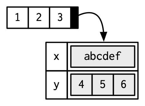
#> [26]  1

Lists

sometimes called a generic vector or recursive vector
Recall (section 2.3.3): each element is really a reference to another object
an be composed of elements of different types (as opposed to atomic vectors which must be of only one type)

Constructing

Simple lists:

# Construct
simple_list <- list(
  c(TRUE, FALSE),   # logicals
  1:20,             # integers
  c(1.2, 2.3, 3.4), # doubles
  c("primo", "secundo", "tercio") # characters
)

simple_list

#> [[1]]
#> [1]  TRUE FALSE
#> 
#> [[2]]
#>  [1]  1  2  3  4  5  6  7  8  9 10 11 12 13 14 15 16 17 18 19 20
#> 
#> [[3]]
#> [1] 1.2 2.3 3.4
#> 
#> [[4]]
#> [1] "primo"   "secundo" "tercio"

# Inspect
# - type
typeof(simple_list)

#> [1] "list"

# - structure
str(simple_list)

#> List of 4
#>  $ : logi [1:2] TRUE FALSE
#>  $ : int [1:20] 1 2 3 4 5 6 7 8 9 10 ...
#>  $ : num [1:3] 1.2 2.3 3.4
#>  $ : chr [1:3] "primo" "secundo" "tercio"

# Accessing
simple_list[1]

#> [[1]]
#> [1]  TRUE FALSE

simple_list[2]

#> [[1]]
#>  [1]  1  2  3  4  5  6  7  8  9 10 11 12 13 14 15 16 17 18 19 20

simple_list[3]

#> [[1]]
#> [1] 1.2 2.3 3.4

simple_list[4]

#> [[1]]
#> [1] "primo"   "secundo" "tercio"

simple_list[[1]][2]

#> [1] FALSE

simple_list[[2]][8]

#> [1] 8

simple_list[[3]][2]

#> [1] 2.3

simple_list[[4]][3]

#> [1] "tercio"

Even Simpler List

# Construct
simpler_list <- list(TRUE, FALSE, 
                    1, 2, 3, 4, 5, 
                    1.2, 2.3, 3.4, 
                    "primo", "secundo", "tercio")

# Accessing
simpler_list[1]

#> [[1]]
#> [1] TRUE

simpler_list[5]

#> [[1]]
#> [1] 3

simpler_list[9]

#> [[1]]
#> [1] 2.3

simpler_list[11]

#> [[1]]
#> [1] "primo"

Nested lists:

nested_list <- list(
  # first level
  list(
    # second level
    list(
      # third level
      list(1)
    )
  )
)

str(nested_list)

#> List of 1
#>  $ :List of 1
#>   ..$ :List of 1
#>   .. ..$ :List of 1
#>   .. .. ..$ : num 1

Like JSON.

Combined lists

list_comb1 <- list(list(1, 2), list(3, 4)) # with list()
list_comb2 <- c(list(1, 2), list(3, 4)) # with c()

# compare structure
str(list_comb1)

#> List of 2
#>  $ :List of 2
#>   ..$ : num 1
#>   ..$ : num 2
#>  $ :List of 2
#>   ..$ : num 3
#>   ..$ : num 4

str(list_comb2)

#> List of 4
#>  $ : num 1
#>  $ : num 2
#>  $ : num 3
#>  $ : num 4

# does this work if they are different data types?
list_comb3 <- c(list(1, 2), list(TRUE, FALSE))
str(list_comb3)

#> List of 4
#>  $ : num 1
#>  $ : num 2
#>  $ : logi TRUE
#>  $ : logi FALSE

Testing

Check that is a list:

is.list()
`rlang::is_list()``

The two do the same, except that the latter can check for the number of elements

# is list
base::is.list(list_comb2)

#> [1] TRUE

rlang::is_list(list_comb2)

#> [1] TRUE

# is list of 4 elements
rlang::is_list(x = list_comb2, n = 4)

#> [1] TRUE

# is a vector (of a special type)
# remember the family tree?
rlang::is_vector(list_comb2)

#> [1] TRUE

Coercion

Use as.list()

list(1:3)

#> [[1]]
#> [1] 1 2 3

as.list(1:3)

#> [[1]]
#> [1] 1
#> 
#> [[2]]
#> [1] 2
#> 
#> [[3]]
#> [1] 3

Matrices and arrays

Although not often used, the dimension attribute can be added to create list-matrices or list-arrays.

l <- list(1:3, "a", TRUE, 1.0)
dim(l) <- c(2, 2); l

#>      [,1]      [,2]
#> [1,] integer,3 TRUE
#> [2,] "a"       1

l[[1, 1]]

#> [1] 1 2 3

Exercises 1/3

List all the ways that a list differs from an atomic vector.

Answer(s)

Atomic vectors are always homogeneous (all elements must be of the same type). Lists may be heterogeneous (the elements can be of different types) as described in the introduction of the vectors chapter.
Atomic vectors point to one address in memory, while lists contain a separate reference for each element. (This was described in the list sections of the vectors and the names and values chapters.)

lobstr::ref(1:2)
#> [1:0x7fcd936f6e80] <int>
lobstr::ref(list(1:2, 2))
#> █ [1:0x7fcd93d53048] <list> 
#> ├─[2:0x7fcd91377e40] <int> 
#> └─[3:0x7fcd93b41eb0] <dbl>

Subsetting with out-of-bounds and NA values leads to different output. For example, [ returns NA for atomics and NULL for lists. (This is described in more detail within the subsetting chapter.)

# Subsetting atomic vectors
(1:2)[3]
#> [1] NA
(1:2)[NA]
#> [1] NA NA

# Subsetting lists
as.list(1:2)[3]
#> [[1]]
#> NULL
as.list(1:2)[NA]
#> [[1]]
#> NULL
#> 
#> [[2]]
#> NULL

Exercises 2/3

Why do you need to use unlist() to convert a list to an atomic vector? Why doesn’t as.vector() work?

Answer(s)

A list is already a vector, though not an atomic one! Note that as.vector() and is.vector() use different definitions of “vector!”

is.vector(as.vector(mtcars))
#> [1] FALSE

Exercises 3/3

Compare and contrast c() and unlist() when combining a date and date-time into a single vector.

Answer(s)

Date and date-time objects are both built upon doubles. While dates store the number of days since the reference date 1970-01-01 (also known as “the Epoch”) in days, date-time-objects (POSIXct) store the time difference to this date in seconds.

date    <- as.Date("1970-01-02")
dttm_ct <- as.POSIXct("1970-01-01 01:00", tz = "UTC")

# Internal representations
unclass(date)
#> [1] 1
unclass(dttm_ct)
#> [1] 3600
#> attr(,"tzone")
#> [1] "UTC"

As the c() generic only dispatches on its first argument, combining date and date-time objects via c() could lead to surprising results in older R versions (pre R 4.0.0):

# Output in R version 3.6.2
c(date, dttm_ct)  # equal to c.Date(date, dttm_ct) 
#> [1] "1970-01-02" "1979-11-10"
c(dttm_ct, date)  # equal to c.POSIXct(date, dttm_ct)
#> [1] "1970-01-01 02:00:00 CET" "1970-01-01 01:00:01 CET"

In the first statement above c.Date() is executed, which incorrectly treats the underlying double of dttm_ct (3600) as days instead of seconds. Conversely, when c.POSIXct() is called on a date, one day is counted as one second only.

We can highlight these mechanics by the following code:

# Output in R version 3.6.2
unclass(c(date, dttm_ct))  # internal representation
#> [1] 1 3600
date + 3599
#> "1979-11-10"

As of R 4.0.0 these issues have been resolved and both methods now convert their input first into POSIXct and Date, respectively.

c(dttm_ct, date)
#> [1] "1970-01-01 01:00:00 UTC" "1970-01-02 00:00:00 UTC"
unclass(c(dttm_ct, date))
#> [1]  3600 86400

c(date, dttm_ct)
#> [1] "1970-01-02" "1970-01-01"
unclass(c(date, dttm_ct))
#> [1] 1 0

However, as c() strips the time zone (and other attributes) of POSIXct objects, some caution is still recommended.

(dttm_ct <- as.POSIXct("1970-01-01 01:00", tz = "HST"))
#> [1] "1970-01-01 01:00:00 HST"
attributes(c(dttm_ct))
#> $class
#> [1] "POSIXct" "POSIXt"

A package that deals with these kinds of problems in more depth and provides a structural solution for them is the {vctrs} package9 which is also used throughout the tidyverse.10

Let’s look at unlist(), which operates on list input.

# Attributes are stripped
unlist(list(date, dttm_ct))  
#> [1]     1 39600

We see again that dates and date-times are internally stored as doubles. Unfortunately, this is all we are left with, when unlist strips the attributes of the list.

To summarise: c() coerces types and strips time zones. Errors may have occurred in older R versions because of inappropriate method dispatch/immature methods. unlist() strips attributes.

Data frames and tibbles

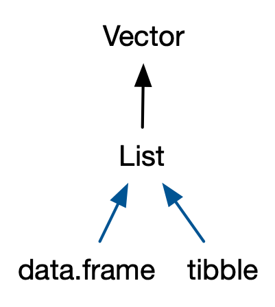
Credit: Advanced R by Hadley Wickham

Data frame

A data frame is a:

Named list of vectors (i.e., column names)
Attributes:
- (column) names
- row.names
- Class: “data frame”

Data frame, examples 1/2:

# Construct
df <- data.frame(
  col1 = c(1, 2, 3),              # named atomic vector
  col2 = c("un", "deux", "trois") # another named atomic vector
  # ,stringsAsFactors = FALSE # default for versions after R 4.1
)
# Inspect
df

#>   col1  col2
#> 1    1    un
#> 2    2  deux
#> 3    3 trois

# Deconstruct
# - type
typeof(df)

#> [1] "list"

# - attributes
attributes(df)

#> $names
#> [1] "col1" "col2"
#> 
#> $class
#> [1] "data.frame"
#> 
#> $row.names
#> [1] 1 2 3

Data frame, examples 2/2:

rownames(df)

#> [1] "1" "2" "3"

colnames(df)

#> [1] "col1" "col2"

names(df) # Same as colnames(df)

#> [1] "col1" "col2"

nrow(df)

#> [1] 3

ncol(df)

#> [1] 2

length(df) # Same as ncol(df)

#> [1] 2

Unlike other lists, the length of each vector must be the same (i.e. as many vector elements as rows in the data frame).

Tibble

Created to relieve some of the frustrations and pain points created by data frames, tibbles are data frames that are:

Lazy (do less)
Surly (complain more)

Lazy

Tibbles do not:

Coerce strings
Transform non-syntactic names
Recycle vectors of length greater than 1

! Coerce strings

chr_col <- c("don't", "factor", "me", "bro")

# data frame
df <- data.frame(
  a = chr_col,
  # in R 4.1 and earlier, this was the default
  stringsAsFactors = TRUE
)

# tibble
tbl <- tibble::tibble(
  a = chr_col
)

# contrast the structure
str(df$a)

#>  Factor w/ 4 levels "bro","don't",..: 2 3 4 1

str(tbl$a)

#>  chr [1:4] "don't" "factor" "me" "bro"

! Transform non-syntactic names

# data frame
df <- data.frame(
  `1` = c(1, 2, 3)
)

# tibble
tbl <- tibble::tibble(
  `1` = c(1, 2, 3)
)

# contrast the names
names(df)

#> [1] "X1"

names(tbl)

#> [1] "1"

! Recycle vectors of length greater than 1

# data frame
df <- data.frame(
  col1 = c(1, 2, 3, 4),
  col2 = c(1, 2)
)

# tibble
tbl <- tibble::tibble(
  col1 = c(1, 2, 3, 4),
  col2 = c(1, 2)
)

#> Error in `tibble::tibble()`:
#> ! Tibble columns must have compatible sizes.
#> • Size 4: Existing data.
#> • Size 2: Column `col2`.
#> ℹ Only values of size one are recycled.

Surly

Tibbles do only what they’re asked and complain if what they’re asked doesn’t make sense:

Subsetting always yields a tibble
Complains if cannot find column

Subsetting always yields a tibble

# data frame
df <- data.frame(
  col1 = c(1, 2, 3, 4)
)

# tibble
tbl <- tibble::tibble(
  col1 = c(1, 2, 3, 4)
)

# contrast
df_col <- df[, "col1"]
str(df_col)

#>  num [1:4] 1 2 3 4

tbl_col <- tbl[, "col1"]
str(tbl_col)

#> tibble [4 × 1] (S3: tbl_df/tbl/data.frame)
#>  $ col1: num [1:4] 1 2 3 4

# to select a vector, do one of these instead
tbl_col_1 <- tbl[["col1"]]
str(tbl_col_1)

#>  num [1:4] 1 2 3 4

tbl_col_2 <- dplyr::pull(tbl, col1)
str(tbl_col_2)

#>  num [1:4] 1 2 3 4

Complains if cannot find column

names(df)

#> [1] "col1"

df$col

#> [1] 1 2 3 4

names(tbl)

#> [1] "col1"

tbl$col

#> Warning: Unknown or uninitialised column: `col`.

#> NULL

One more difference

tibble() allows you to refer to variables created during construction

tibble::tibble(
  x = 1:3,
  y = x * 2 # x refers to the line above
)

#> # A tibble: 3 × 2
#>       x     y
#>   <int> <dbl>
#> 1     1     2
#> 2     2     4
#> 3     3     6

Side Quest: Row Names

character vector containing only unique values
get and set with rownames()
can use them to subset rows

df3 <- data.frame(
  age = c(35, 27, 18),
  hair = c("blond", "brown", "black"),
  row.names = c("Bob", "Susan", "Sam")
)
df3

#>       age  hair
#> Bob    35 blond
#> Susan  27 brown
#> Sam    18 black

rownames(df3)

#> [1] "Bob"   "Susan" "Sam"

df3["Bob", ]

#>     age  hair
#> Bob  35 blond

rownames(df3) <- c("Susan", "Bob", "Sam")
rownames(df3)

#> [1] "Susan" "Bob"   "Sam"

df3["Bob", ]

#>     age  hair
#> Bob  27 brown

There are three reasons why row names are undesirable:

Metadata is data, so storing it in a different way to the rest of the data is fundamentally a bad idea.
Row names are a poor abstraction for labelling rows because they only work when a row can be identified by a single string. This fails in many cases.
Row names must be unique, so any duplication of rows (e.g. from bootstrapping) will create new row names.

Tibles: Printing

Data frames and tibbles print differently

df3

#>       age  hair
#> Susan  35 blond
#> Bob    27 brown
#> Sam    18 black

tibble::as_tibble(df3)

#> # A tibble: 3 × 2
#>     age hair 
#>   <dbl> <chr>
#> 1    35 blond
#> 2    27 brown
#> 3    18 black

Tibles: Subsetting

Two undesirable subsetting behaviours:

When you subset columns with df[, vars], you will get a vector if vars selects one variable, otherwise you’ll get a data frame, unless you always remember to use df[, vars, drop = FALSE].
When you attempt to extract a single column with df$x and there is no column x, a data frame will instead select any variable that starts with x. If no variable starts with x, df$x will return NULL.

Tibbles tweak these behaviours so that a [ always returns a tibble, and a $ doesn’t do partial matching and warns if it can’t find a variable (this is what makes tibbles surly).

Tibles: Testing

Whether data frame: is.data.frame(). Note: both data frame and tibble are data frames.

Whether tibble: tibble::is_tibble. Note: only tibbles are tibbles. Vanilla data frames are not.

Tibles: Coercion

To data frame: as.data.frame()
To tibble: tibble::as_tibble()

Tibles: List Columns

List-columns are allowed in data frames but you have to do a little extra work by either adding the list-column after creation or wrapping the list in I()

df4 <- data.frame(x = 1:3)
df4$y <- list(1:2, 1:3, 1:4)
df4

#>   x          y
#> 1 1       1, 2
#> 2 2    1, 2, 3
#> 3 3 1, 2, 3, 4

df5 <- data.frame(
  x = 1:3, 
  y = I(list(1:2, 1:3, 1:4))
)
df5

#>   x          y
#> 1 1       1, 2
#> 2 2    1, 2, 3
#> 3 3 1, 2, 3, 4

Tibbles: Matrix and data frame columns

As long as the number of rows matches the data frame, it’s also possible to have a matrix or data frame as a column of a data frame.
same as list-columns, must either addi the list-column after creation or wrapping the list in I()

dfm <- data.frame(
  x = 1:3 * 10,
  y = I(matrix(1:9, nrow = 3))
)

dfm$z <- data.frame(a = 3:1, b = letters[1:3], stringsAsFactors = FALSE)

str(dfm)

#> 'data.frame':    3 obs. of  3 variables:
#>  $ x: num  10 20 30
#>  $ y: 'AsIs' int [1:3, 1:3] 1 2 3 4 5 6 7 8 9
#>  $ z:'data.frame':   3 obs. of  2 variables:
#>   ..$ a: int  3 2 1
#>   ..$ b: chr  "a" "b" "c"

dfm$y

#>      [,1] [,2] [,3]
#> [1,]    1    4    7
#> [2,]    2    5    8
#> [3,]    3    6    9

dfm$z

#>   a b
#> 1 3 a
#> 2 2 b
#> 3 1 c

Exercises 1/4

Can you have a data frame with zero rows? What about zero columns?

Answer(s)

Yes, you can create these data frames easily; either during creation or via subsetting. Even both dimensions can be zero. Create a 0-row, 0-column, or an empty data frame directly:

data.frame(a = integer(), b = logical())
#> [1] a b
#> <0 rows> (or 0-length row.names)

data.frame(row.names = 1:3)  # or data.frame()[1:3, ]
#> data frame with 0 columns and 3 rows

data.frame()
#> data frame with 0 columns and 0 rows

Create similar data frames via subsetting the respective dimension with either 0, NULL, FALSE or a valid 0-length atomic (logical(0), character(0), integer(0), double(0)). Negative integer sequences would also work. The following example uses a zero:

mtcars[0, ]
#>  [1] mpg  cyl  disp hp   drat wt   qsec vs   am   gear carb
#> <0 rows> (or 0-length row.names)

mtcars[ , 0]  # or mtcars[0]
#> data frame with 0 columns and 32 rows

mtcars[0, 0]
#> data frame with 0 columns and 0 rows

Exercises 2/4

What happens if you attempt to set rownames that are not unique?

Answer(s)

Matrices can have duplicated row names, so this does not cause problems.

Data frames, however, require unique rownames and you get different results depending on how you attempt to set them. If you set them directly or via row.names(), you get an error:

data.frame(row.names = c("x", "y", "y"))
#> Error in data.frame(row.names = c("x", "y", "y")): duplicate row.names: y

df <- data.frame(x = 1:3)
row.names(df) <- c("x", "y", "y")
#> Warning: non-unique value when setting 'row.names': 'y'
#> Error in `.rowNamesDF<-`(x, value = value): duplicate 'row.names' are not allowed

If you use subsetting, [ automatically deduplicates:

row.names(df) <- c("x", "y", "z")
df[c(1, 1, 1), , drop = FALSE]
#>     x
#> x   1
#> x.1 1
#> x.2 1

Exercises 3/4

If df is a data frame, what can you say about t(df), and t(t(df))? Perform some experiments, making sure to try different column types.

Answer(s)

Both of t(df) and t(t(df)) will return matrices:

df <- data.frame(x = 1:3, y = letters[1:3])
is.matrix(df)
#> [1] FALSE
is.matrix(t(df))
#> [1] TRUE
is.matrix(t(t(df)))
#> [1] TRUE

The dimensions will respect the typical transposition rules:

dim(df)
#> [1] 3 2
dim(t(df))
#> [1] 2 3
dim(t(t(df)))
#> [1] 3 2

Because the output is a matrix, every column is coerced to the same type. (It is implemented within t.data.frame() via as.matrix() which is described below).

df
#>   x y
#> 1 1 a
#> 2 2 b
#> 3 3 c
t(df)
#>   [,1] [,2] [,3]
#> x "1"  "2"  "3" 
#> y "a"  "b"  "c"

Exercises 4/4

What does as.matrix() do when applied to a data frame with columns of different types? How does it differ from data.matrix()?

Answer(s)

The type of the result of as.matrix depends on the types of the input columns (see ?as.matrix):

The method for data frames will return a character matrix if there is only atomic columns and any non-(numeric/logical/complex) column, applying as.vector to factors and format to other non-character columns. Otherwise the usual coercion hierarchy (logical < integer < double < complex) will be used, e.g. all-logical data frames will be coerced to a logical matrix, mixed logical-integer will give an integer matrix, etc.

On the other hand, data.matrix will always return a numeric matrix (see ?data.matrix()).

Return the matrix obtained by converting all the variables in a data frame to numeric mode and then binding them together as the columns of a matrix. Factors and ordered factors are replaced by their internal codes. […] Character columns are first converted to factors and then to integers.

We can illustrate and compare the mechanics of these functions using a concrete example. as.matrix() makes it possible to retrieve most of the original information from the data frame but leaves us with characters. To retrieve all information from data.matrix()’s output, we would need a lookup table for each column.

df_coltypes <- data.frame(
  a = c("a", "b"),
  b = c(TRUE, FALSE),
  c = c(1L, 0L),
  d = c(1.5, 2),
  e = factor(c("f1", "f2"))
)

as.matrix(df_coltypes)
#>      a   b       c   d     e   
#> [1,] "a" "TRUE"  "1" "1.5" "f1"
#> [2,] "b" "FALSE" "0" "2.0" "f2"
data.matrix(df_coltypes)
#>      a b c   d e
#> [1,] 1 1 1 1.5 1
#> [2,] 2 0 0 2.0 2

`NULL`

Special type of object that:

Length 0
Cannot have attributes

typeof(NULL)
#> [1] "NULL"

length(NULL)
#> [1] 0

x <- NULL
attr(x, "y") <- 1

#> Error in attr(x, "y") <- 1: attempt to set an attribute on NULL

is.null(NULL)

#> [1] TRUE

Digestif

Let is use some of this chapter’s skills on the penguins data.

Attributes

str(penguins_raw)

#> tibble [344 × 17] (S3: tbl_df/tbl/data.frame)
#>  $ studyName          : chr [1:344] "PAL0708" "PAL0708" "PAL0708" "PAL0708" ...
#>  $ Sample Number      : num [1:344] 1 2 3 4 5 6 7 8 9 10 ...
#>  $ Species            : chr [1:344] "Adelie Penguin (Pygoscelis adeliae)" "Adelie Penguin (Pygoscelis adeliae)" "Adelie Penguin (Pygoscelis adeliae)" "Adelie Penguin (Pygoscelis adeliae)" ...
#>  $ Region             : chr [1:344] "Anvers" "Anvers" "Anvers" "Anvers" ...
#>  $ Island             : chr [1:344] "Torgersen" "Torgersen" "Torgersen" "Torgersen" ...
#>  $ Stage              : chr [1:344] "Adult, 1 Egg Stage" "Adult, 1 Egg Stage" "Adult, 1 Egg Stage" "Adult, 1 Egg Stage" ...
#>  $ Individual ID      : chr [1:344] "N1A1" "N1A2" "N2A1" "N2A2" ...
#>  $ Clutch Completion  : chr [1:344] "Yes" "Yes" "Yes" "Yes" ...
#>  $ Date Egg           : Date[1:344], format: "2007-11-11" "2007-11-11" ...
#>  $ Culmen Length (mm) : num [1:344] 39.1 39.5 40.3 NA 36.7 39.3 38.9 39.2 34.1 42 ...
#>  $ Culmen Depth (mm)  : num [1:344] 18.7 17.4 18 NA 19.3 20.6 17.8 19.6 18.1 20.2 ...
#>  $ Flipper Length (mm): num [1:344] 181 186 195 NA 193 190 181 195 193 190 ...
#>  $ Body Mass (g)      : num [1:344] 3750 3800 3250 NA 3450 ...
#>  $ Sex                : chr [1:344] "MALE" "FEMALE" "FEMALE" NA ...
#>  $ Delta 15 N (o/oo)  : num [1:344] NA 8.95 8.37 NA 8.77 ...
#>  $ Delta 13 C (o/oo)  : num [1:344] NA -24.7 -25.3 NA -25.3 ...
#>  $ Comments           : chr [1:344] "Not enough blood for isotopes." NA NA "Adult not sampled." ...
#>  - attr(*, "spec")=List of 3
#>   ..$ cols   :List of 17
#>   .. ..$ studyName          : list()
#>   .. .. ..- attr(*, "class")= chr [1:2] "collector_character" "collector"
#>   .. ..$ Sample Number      : list()
#>   .. .. ..- attr(*, "class")= chr [1:2] "collector_double" "collector"
#>   .. ..$ Species            : list()
#>   .. .. ..- attr(*, "class")= chr [1:2] "collector_character" "collector"
#>   .. ..$ Region             : list()
#>   .. .. ..- attr(*, "class")= chr [1:2] "collector_character" "collector"
#>   .. ..$ Island             : list()
#>   .. .. ..- attr(*, "class")= chr [1:2] "collector_character" "collector"
#>   .. ..$ Stage              : list()
#>   .. .. ..- attr(*, "class")= chr [1:2] "collector_character" "collector"
#>   .. ..$ Individual ID      : list()
#>   .. .. ..- attr(*, "class")= chr [1:2] "collector_character" "collector"
#>   .. ..$ Clutch Completion  : list()
#>   .. .. ..- attr(*, "class")= chr [1:2] "collector_character" "collector"
#>   .. ..$ Date Egg           :List of 1
#>   .. .. ..$ format: chr ""
#>   .. .. ..- attr(*, "class")= chr [1:2] "collector_date" "collector"
#>   .. ..$ Culmen Length (mm) : list()
#>   .. .. ..- attr(*, "class")= chr [1:2] "collector_double" "collector"
#>   .. ..$ Culmen Depth (mm)  : list()
#>   .. .. ..- attr(*, "class")= chr [1:2] "collector_double" "collector"
#>   .. ..$ Flipper Length (mm): list()
#>   .. .. ..- attr(*, "class")= chr [1:2] "collector_double" "collector"
#>   .. ..$ Body Mass (g)      : list()
#>   .. .. ..- attr(*, "class")= chr [1:2] "collector_double" "collector"
#>   .. ..$ Sex                : list()
#>   .. .. ..- attr(*, "class")= chr [1:2] "collector_character" "collector"
#>   .. ..$ Delta 15 N (o/oo)  : list()
#>   .. .. ..- attr(*, "class")= chr [1:2] "collector_double" "collector"
#>   .. ..$ Delta 13 C (o/oo)  : list()
#>   .. .. ..- attr(*, "class")= chr [1:2] "collector_double" "collector"
#>   .. ..$ Comments           : list()
#>   .. .. ..- attr(*, "class")= chr [1:2] "collector_character" "collector"
#>   ..$ default: list()
#>   .. ..- attr(*, "class")= chr [1:2] "collector_guess" "collector"
#>   ..$ skip   : num 1
#>   ..- attr(*, "class")= chr "col_spec"

str(penguins_raw, give.attr = FALSE)

#> tibble [344 × 17] (S3: tbl_df/tbl/data.frame)
#>  $ studyName          : chr [1:344] "PAL0708" "PAL0708" "PAL0708" "PAL0708" ...
#>  $ Sample Number      : num [1:344] 1 2 3 4 5 6 7 8 9 10 ...
#>  $ Species            : chr [1:344] "Adelie Penguin (Pygoscelis adeliae)" "Adelie Penguin (Pygoscelis adeliae)" "Adelie Penguin (Pygoscelis adeliae)" "Adelie Penguin (Pygoscelis adeliae)" ...
#>  $ Region             : chr [1:344] "Anvers" "Anvers" "Anvers" "Anvers" ...
#>  $ Island             : chr [1:344] "Torgersen" "Torgersen" "Torgersen" "Torgersen" ...
#>  $ Stage              : chr [1:344] "Adult, 1 Egg Stage" "Adult, 1 Egg Stage" "Adult, 1 Egg Stage" "Adult, 1 Egg Stage" ...
#>  $ Individual ID      : chr [1:344] "N1A1" "N1A2" "N2A1" "N2A2" ...
#>  $ Clutch Completion  : chr [1:344] "Yes" "Yes" "Yes" "Yes" ...
#>  $ Date Egg           : Date[1:344], format: "2007-11-11" "2007-11-11" ...
#>  $ Culmen Length (mm) : num [1:344] 39.1 39.5 40.3 NA 36.7 39.3 38.9 39.2 34.1 42 ...
#>  $ Culmen Depth (mm)  : num [1:344] 18.7 17.4 18 NA 19.3 20.6 17.8 19.6 18.1 20.2 ...
#>  $ Flipper Length (mm): num [1:344] 181 186 195 NA 193 190 181 195 193 190 ...
#>  $ Body Mass (g)      : num [1:344] 3750 3800 3250 NA 3450 ...
#>  $ Sex                : chr [1:344] "MALE" "FEMALE" "FEMALE" NA ...
#>  $ Delta 15 N (o/oo)  : num [1:344] NA 8.95 8.37 NA 8.77 ...
#>  $ Delta 13 C (o/oo)  : num [1:344] NA -24.7 -25.3 NA -25.3 ...
#>  $ Comments           : chr [1:344] "Not enough blood for isotopes." NA NA "Adult not sampled." ...

Data Frames vs Tibbles

penguins_df <- data.frame(penguins)
penguins_tb <- penguins #i.e. penguins was already a tibble

Printing

Tip: print out these results in RStudio under different editor themes

print(penguins_df) #don't run this

head(penguins_df)

#>   species    island bill_length_mm bill_depth_mm flipper_length_mm body_mass_g
#> 1  Adelie Torgersen           39.1          18.7               181        3750
#> 2  Adelie Torgersen           39.5          17.4               186        3800
#> 3  Adelie Torgersen           40.3          18.0               195        3250
#> 4  Adelie Torgersen             NA            NA                NA          NA
#> 5  Adelie Torgersen           36.7          19.3               193        3450
#> 6  Adelie Torgersen           39.3          20.6               190        3650
#>      sex year
#> 1   male 2007
#> 2 female 2007
#> 3 female 2007
#> 4   <NA> 2007
#> 5 female 2007
#> 6   male 2007

penguins_tb

#> # A tibble: 344 × 8
#>    species island    bill_length_mm bill_depth_mm flipper_length_mm body_mass_g
#>    <fct>   <fct>              <dbl>         <dbl>             <int>       <int>
#>  1 Adelie  Torgersen           39.1          18.7               181        3750
#>  2 Adelie  Torgersen           39.5          17.4               186        3800
#>  3 Adelie  Torgersen           40.3          18                 195        3250
#>  4 Adelie  Torgersen           NA            NA                  NA          NA
#>  5 Adelie  Torgersen           36.7          19.3               193        3450
#>  6 Adelie  Torgersen           39.3          20.6               190        3650
#>  7 Adelie  Torgersen           38.9          17.8               181        3625
#>  8 Adelie  Torgersen           39.2          19.6               195        4675
#>  9 Adelie  Torgersen           34.1          18.1               193        3475
#> 10 Adelie  Torgersen           42            20.2               190        4250
#> # ℹ 334 more rows
#> # ℹ 2 more variables: sex <fct>, year <int>

Atomic Vectors

species_vector_df <- penguins_df |> select(species)
species_unlist_df <- penguins_df |> select(species) |> unlist()
species_pull_df   <- penguins_df |> select(species) |> pull()

species_vector_tb <- penguins_tb |> select(species)
species_unlist_tb <- penguins_tb |> select(species) |> unlist()
species_pull_tb   <- penguins_tb |> select(species) |> pull()

typeof() and class()

typeof(species_vector_df)

#> [1] "list"

class(species_vector_df)

#> [1] "data.frame"

typeof(species_unlist_df)

#> [1] "integer"

class(species_unlist_df)

#> [1] "factor"

typeof(species_pull_df)

#> [1] "integer"

class(species_pull_df)

#> [1] "factor"

typeof(species_vector_tb)

#> [1] "list"

class(species_vector_tb)

#> [1] "tbl_df"     "tbl"        "data.frame"

typeof(species_unlist_tb)

#> [1] "integer"

class(species_unlist_tb)

#> [1] "factor"

typeof(species_pull_tb)

#> [1] "integer"

class(species_pull_tb)

#> [1] "factor"

Column Names

colnames(penguins_tb)

#> [1] "species"           "island"            "bill_length_mm"   
#> [4] "bill_depth_mm"     "flipper_length_mm" "body_mass_g"      
#> [7] "sex"               "year"

names(penguins_tb) == colnames(penguins_tb)

#> [1] TRUE TRUE TRUE TRUE TRUE TRUE TRUE TRUE

names(penguins_df) == names(penguins_tb)

#> [1] TRUE TRUE TRUE TRUE TRUE TRUE TRUE TRUE

What if we only invoke a partial name of a column of a tibble?

penguins_tb$y

#> NULL

tibbles are surly!

What if we only invoke a partial name of a column of a data frame?

head(penguins_df$y) #instead of `year`

#> [1] 2007 2007 2007 2007 2007 2007

Is this evaluation in alphabetical order or column order?

penguins_df_se_sp <- penguins_df |> select(sex, species)
penguins_df_sp_se <- penguins_df |> select(species, sex)

head(penguins_df_se_sp$s)

#> NULL

head(penguins_df_sp_se$s)

#> NULL

Chapter Quiz 1/5

What are the four common types of atomic vectors? What are the two rare types?

Answer(s)

The four common types of atomic vector are logical, integer, double and character. The two rarer types are complex and raw.

Chapter Quiz 2/5

What are attributes? How do you get them and set them?

Answer(s)

Attributes allow you to associate arbitrary additional metadata to any object. You can get and set individual attributes with attr(x, "y") and attr(x, "y") <- value; or you can get and set all attributes at once with attributes().

Chapter Quiz 3/5

How is a list different from an atomic vector? How is a matrix different from a data frame?

Answer(s)

The elements of a list can be any type (even a list); the elements of an atomic vector are all of the same type. Similarly, every element of a matrix must be the same type; in a data frame, different columns can have different types.

Chapter Quiz 4/5

Can you have a list that is a matrix? Can a data frame have a column that is a matrix?

Answer(s)

You can make a list-array by assigning dimensions to a list. You can make a matrix a column of a data frame with df$x <- matrix(), or by using I() when creating a new data frame data.frame(x = I(matrix())).

Chapter Quiz 5/5

How do tibbles behave differently from data frames?

Answer(s)

Tibbles have an enhanced print method, never coerce strings to factors, and provide stricter subsetting methods.

Vectors

Learning objectives:

Session Info

Aperitif

Counting Penguins

In

Fix: base R

Fix: dplyr

Motivation

Types of Vectors

Types of Atomic Vectors (1/2)

Types of Atomic Vectors (2/2)

Vectors of Length One

Logicals

Doubles

Integers

Strings

Longer 1/2

Longer 2/2

Type and Length

Side Quest: Penguins

Missing values: Contagion

Missing values: Contagion Exceptions

Innoculation

Missing Values: NA Types

Testing (1/2)

Testing (2/2)

Side Quest: rlang is_*()

Coercion

Automatic

Coercion by Combination:

Coercion by Mathematical operations:

Explicit

Exercises 1/5

Exercises 2/5

Exercises 3/5

Exercises 4/5

Exercises 5/5

Attributes

Getting and Setting

Single attribute

Multiple attributes

Why

Names

rlang Names

Removing names

Dimensions: matrix() and array()

Dimensions: assign to dim()

Functions for working with vectors, matrices and arrays (1/2):

Functions for working with vectors, matrices and arrays (2/2):

Exercises 1/4

Exercises 1/4 (cont)

Exercises 2/4

Exercises 3/4

Exercises 4/4

Exercises 4/4 (cont)

Class - S3 atomic vectors

Four important S3 vectors used in base R:

Factors

Factors examples

Custom Order

Dates

Dates Unix epoch

Date-times

Dates-times: POSIXct

Durations

Exercises 1/3

Exercises 2/3

Exercises 3/3

Lists

Constructing

Even Simpler List

Nested lists:

Combined lists

Testing

Coercion

Matrices and arrays

Exercises 1/3

Exercises 2/3

Exercises 3/3

Side Quest: rlang `is_*()`

Dimensions: `matrix()` and `array()`

Dimensions: assign to `dim()`

`NULL`